7
$\begingroup$

I do not understand properly what a spline does even in a simple situation of a piecewise regression, and I need some help. Consider the following basic example:


library(data.table)
df <- data.table(power = seq(50,250,12))

thres1 <- 120
thres2 <- 200
coef1 <- 1/10
coef2 <- 1/5

df[,lactate_raw := fcase(power < thres1,1,
                           power %between% c(thres1,thres2), 1+ (power - thres1)*coef1,
                           power > thres2, 1+ (thres2 - thres1)*coef1 + (power - thres2)*coef2)]

ggplot(df)+
  geom_line(aes(power,lactate_raw),color = "red")+
  geom_point(aes(power,lactate_raw))+
  theme_bw()+
  geom_vline(xintercept = c(thres1,thres2),linetype = "dotted")+
  labs(y = "Blood lactate (mmol/L)",x = "Power (W)")

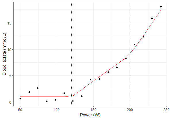
enter image description here

I have data here with three slopes. I can do a simple manual piecewise regression:

fitsimple <- lm(data = df,
                lactate_raw ~ power +
                  I((power - thres1)*(power >= thres1) )+
                  I((power - thres2)*(power >= thres2) ))

Coefficients:
                                        Estimate Std. Error t value Pr(>|t|)    
(Intercept)                              2.36299    1.05772   2.234  0.04368 *  
power                                   -0.01566    0.01126  -1.392  0.18737    
I((power - thres1) * (power >= thres1))  0.12154    0.01839   6.610 1.69e-05 ***
I((power - thres2) * (power >= thres2))  0.11392    0.02754   4.137  0.00117 ** 

Here I have simple coefficients that are easy to interpret, and the fit is nice.

enter image description here

If I now want to use the bs function from the library(splines), I should be able to get the same result, giving the knots and specifying the degree equal to $1$. But I don't get what transformation bs does:

library(splines)
fit <- lm(data = df,
   lactate_raw ~ bs(power,knots = c(thres1,thres2),degree = 1)) 

summary(fit)
Coefficients:
                                                  Estimate Std. Error t value Pr(>|t|)    
(Intercept)                                         1.5797     0.5362   2.946   0.0114 *  
bs(power, knots = c(thres1, thres2), degree = 1)1  -1.0965     0.7879  -1.392   0.1874    
bs(power, knots = c(thres1, thres2), degree = 1)2   7.3734     0.6802  10.840 7.01e-08 ***
bs(power, knots = c(thres1, thres2), degree = 1)3  16.6048     0.8392  19.787 4.35e-11 ***

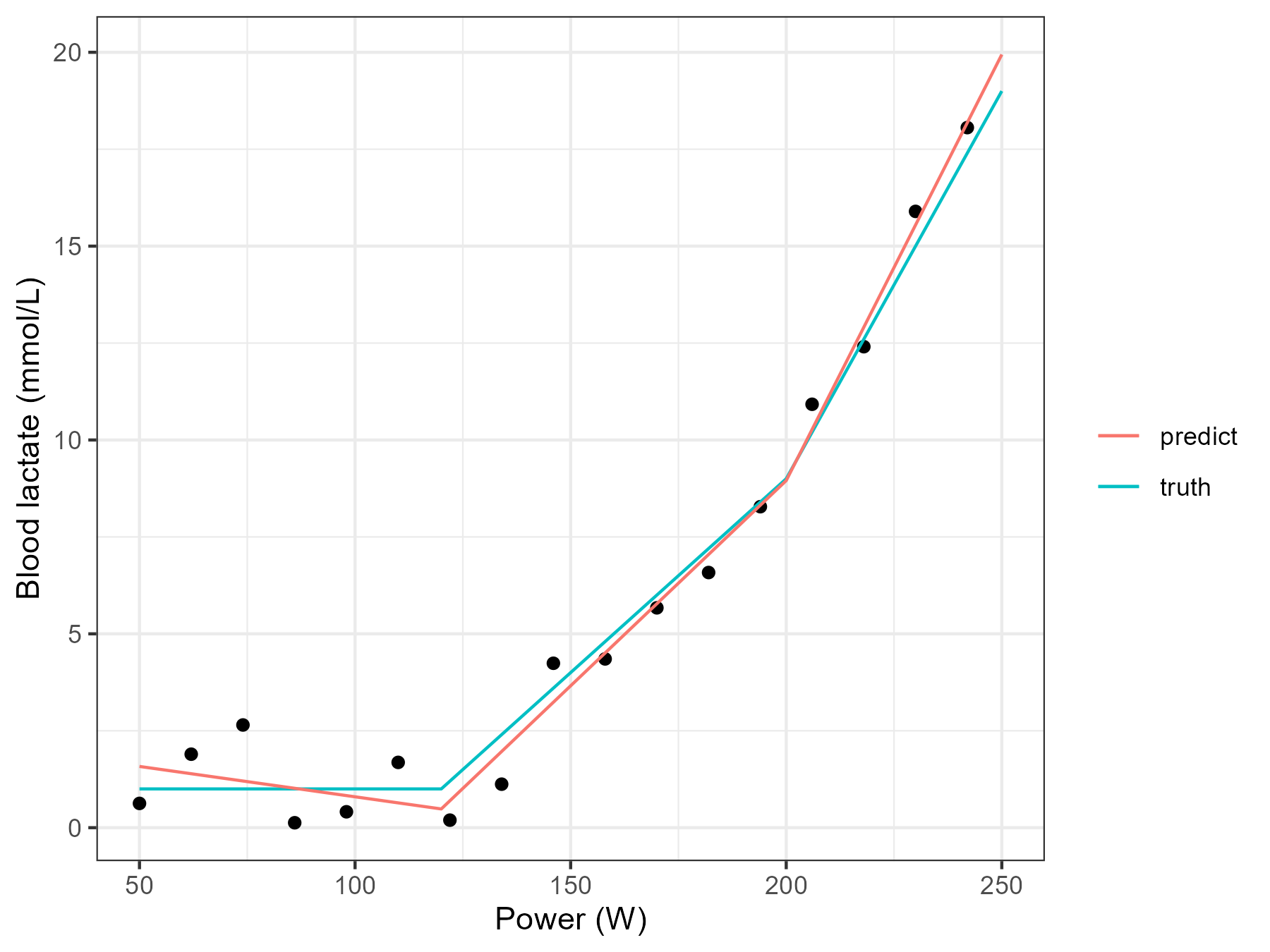
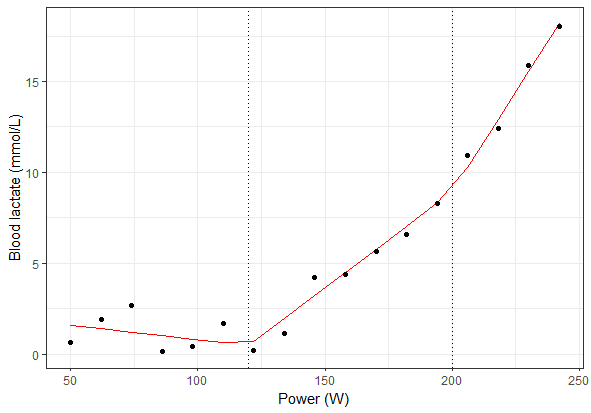
What does these coefficients mean? If I plot the prediction, it does estimate a three-piece linear relation:

df$predict <- predict(fit)
ggplot(df)+
  geom_line(aes(power,predict),color = "red")+
  geom_point(aes(power,lactate_raw))+
  theme_bw()+
  geom_vline(xintercept = c(thres1,thres2),linetype = "dotted")+
  labs(y = "Blood lactate (mmol/L)",x = "Power (W)")

enter image description here

But the transformation of bs has nothing to do with my example by hand.

bs(df$power,knots = c(thres1,thres2),degree = 1) 
              1         2         3
 [1,] 0.0000000 0.0000000 0.0000000
 [2,] 0.1714286 0.0000000 0.0000000
 [3,] 0.3428571 0.0000000 0.0000000
 [4,] 0.5142857 0.0000000 0.0000000
 [5,] 0.6857143 0.0000000 0.0000000
 [6,] 0.8571429 0.0000000 0.0000000
 [7,] 0.9750000 0.0250000 0.0000000
 [8,] 0.8250000 0.1750000 0.0000000
 [9,] 0.6750000 0.3250000 0.0000000
[10,] 0.5250000 0.4750000 0.0000000
[11,] 0.3750000 0.6250000 0.0000000
[12,] 0.2250000 0.7750000 0.0000000
[13,] 0.0750000 0.9250000 0.0000000
[14,] 0.0000000 0.8571429 0.1428571
[15,] 0.0000000 0.5714286 0.4285714
[16,] 0.0000000 0.2857143 0.7142857
[17,] 0.0000000 0.0000000 1.0000000

I do not understand it. Could someone help?

$\endgroup$
6
  • $\begingroup$ one important point is that the spline version is a localized regression and the piecewise linear is not. they extrapolate differently $\endgroup$
    – LudvigH
    Commented Feb 13 at 12:02
  • $\begingroup$ mmmmm Not sure to understand what you say. In my example, both tranform the independent variable in 3 vectors, both produce the same prediction. $\endgroup$
    – denis
    Commented Feb 13 at 13:52
  • 1
    $\begingroup$ Btw I fixed a part of your code which didn't run when I first tried to replicate this. $\endgroup$ Commented Feb 20 at 7:20
  • $\begingroup$ @denis When trying to replicate your code, it appeared that the dependent variable is not generated in the code. Could you provide the exact code you used? $\endgroup$
    – BenP
    Commented Feb 20 at 9:54
  • $\begingroup$ @BenP I thought I fixed all of the code the first time around, but realized there were some bugs I forgot to edit into the question. I fixed all of those now too so the code should work fine now unless I missed something. Just misspelled the same lactate_raw variable throughout the coded sections. $\endgroup$ Commented Feb 21 at 2:12

3 Answers 3

13
+100
$\begingroup$

Conceptual Discussion

Roland seems to present an answer for how one can derive the function based off the programming. I think your core question however remains unanswered...what do the coefficients here in the spline represent? Roland already noted that we don't generally interpret these directly, but it seems you are still confused about what their purpose is based off the comments and your original question, so I will explain to a degree what they do.

First off, coefficients cannot be interpreted the same way as regular $\beta$ coefficients in a regression. Typically a coefficient in linear regression says something like "for every one unit increase in $x$, we get an associated increase in $y$". A B-spline basis behaves very differently and is more for constructing the line than direct interpretation (hence why Roland noted that they're not usually important to look at). The coefficients in a B-spline essentially scale the evaluated basis functions according to the data in order to fit a curve. Each coefficient belongs to a different B-spline basis function. These basis functions are locally defined polynomials of a certain order (shown in the plot from Roland).

Suppose we have a B-spline with $n$ basis functions, $b_1(x), b_2(x),\ldots, b_n(x)$ made up of coefficients $c_1, c_2, \ldots,c_n$. The final spline is made up of a linear equation such that:

$$ S(x) = c_1 b_1(x) + c_2 b_2(x) + \cdots + c_n b_n(x). $$

To summarize this all in one sentence, each coefficient scales the spline different directions by multiplying the coefficients by their bases, in turn giving us our regression line.

Example

It may be easier to see how this is actually working in action. Instead of using your data, I'm going to generate a sequence of values, $x$, and apply a B-spline to them (using default knot placement) and show how changing the coefficients manipulates the regression line. First the data and the bases, which I create with the splines2 package because they have convenient plotting functions:

#### Load Spline Package ####
library(splines2)

#### Define Sequence of X ####
x <- seq(0, 1, length.out = 100)
x

#### Define a B-spline Basis (df = 5) ####
basis <- bSpline(x, df = 5) # same as bs(), but added functionality

Running plot(basis) gives us a quick plot of the 5 estimated basis functions necessary for our regression lines:

enter image description here

We can see that each basis has a minimum and a maximum, with the lines oscillating based on different points of the sequence of $x$. Roland's custom function shows that for your three-piece function this is assembled in the following steps:

  1. First, calculate the third basis function as $b_3 = \frac{x - \text{knot}_2}{\text{max}(x) - \text{knot}_2}$
  2. Then, calculate the second basis function as $b_2 = \frac{x - \text{knot}_1}{\text{knot}_2 - \text{knot}_1} - b_3$
  3. Then, calculate the first basis function as $b_1 = \frac{x - \text{min}(x)}{\text{knot}_1 - \text{min}(x)} - b_2$
  4. For each basis, set the $b = 0$ if $x < \text{knot}_n$. The knots are essentially intervals where the "pieces" of the polynomial meet.

We would just add more steps with more degrees of freedom. If we run head(basis) for our five-piece function, we get an idea of what this is doing in practice:

              1           2            3 4 5
[1,] 0.00000000 0.000000000 0.000000e+00 0 0
[2,] 0.08682556 0.001351903 4.637746e-06 0 0
[3,] 0.16567883 0.005305581 3.710197e-05 0 0
[4,] 0.23685199 0.011707989 1.252191e-04 0 0
[5,] 0.30063723 0.020406081 2.968157e-04 0 0
[6,] 0.35732671 0.031246812 5.797182e-04 0 0

Above are the first 6 rows of values of the five basis functions. Conceptually, we can think of them as "toggle" switches. When they are set to zero, the line for the basis function stays where it is. When it is set to a number, the $y$ value of the basis function shifts upward or downward relative to its last position. You can see the first row is all zeroes, which we see in the plot...all of the basis functions start at zero. But the next five rows illustrate how this toggling works...the first three basis functions increase slightly in value while the last two basis functions are still zero. Again, we can see this in the plot. While the first three colored lines start to elevate, the others remain at zero. These toggles are later used to expand the regression line when multiplied by our estimated coefficients.

Rather than running a regression, let's just make up some coefficients, a set of coefficients that increases and a set of coefficients that decrease.

#### Define Coefficients ####
coefficients1 <- c(1, 2, 3, 4, 5) # increasing line
coefficients2 <- c(5, 4, 3, 2, 1) # decreasing line

Now we just multiply our coefficients by their basis functions by simply using the %*% operator.

#### Compute Splines ####
spline1 <- basis %*% coefficients1
spline1
spline2 <- basis %*% coefficients2
spline2

Notice something...the when printing both the head of both, we see the values both increase!

> head(spline1)
           [,1]
[1,] 0.00000000
[2,] 0.08954327
[3,] 0.17640129
[4,] 0.26064363
[5,] 0.34233984
[6,] 0.42155949
> head(spline2)
          [,1]
[1,] 0.0000000
[2,] 0.4395493
[3,] 0.8497278
[4,] 1.2314676
[5,] 1.5857009
[6,] 1.9133600

But running the tail paints a different picture...the spline continues to increase for the first set of coefficients but decreases for the second set of coefficients:

> tail(spline1)
           [,1]
 [95,] 4.578441
 [96,] 4.657660
 [97,] 4.739356
 [98,] 4.823599
 [99,] 4.910457
[100,] 5.000000
> tail(spline2)
           [,1]
 [95,] 1.421559
 [96,] 1.342340
 [97,] 1.260644
 [98,] 1.176401
 [99,] 1.089543
[100,] 1.000000

Plotting them will make this make more sense:

#### Plot Splines ####
plot(x, # plot x
     spline1, # and the first spline values (basis * coef)
     type = "l", # run a line
     ylim = c(min(spline1, spline2), 
              max(spline1, spline2)), # across the min/max of both splines
     ylab = "Spline", # labels
     xlab = "X", 
     main = "Effect of Coefficients on B-Spline") 

#### Add Other Spline to Plot ####
lines(x, spline2, col = "red")

enter image description here

Now for the million dollar answer to your question: we see that the bases are the same, but the lines shift based off the what coefficient we get. Remember that for the initial values of our basis matrix, the first three basis functions increased, so any multiplier would naturally increase their values (such as we did with our coefficients). But as the basis functions and coefficients shift (such as those we saw for the last values of the matrix), their multiplications result in different adjustments to the spline.

So to reiterate Roland's points in the comments, the coefficients are important, but from an inferential standpoint, they are not all that helpful. All they do is explain to a degree how the lines are constructed.

Addendum

You have probably been secretly asking yourself...how does this work in relation to an actual regression? The coefficients here are arbitrarily estimated after all! Below I show how we put the pieces together. Recall that for OLS, we simply find the coefficients of the predictors by way of the formula:

$$ \beta = (X^T X)^{-1} X^T Y $$

(I explain what this means in a lot more detail in this answer). With our basis functions we are literally doing the same thing, only now we replace the matrix of predictors $X$ with a matrix of our basis functions $B$. Both are still just matrices, we just multiply them in the usual way. We can simulate a normally distributed $y$ outcome variable and fit a regression with our B-splines and then estimate them manually to see how they compare.

#### Load Spline Package ####
library(splines2)
set.seed(123)

#### Define Sequence of X ####
x <- seq(0, 1, length.out = 100)
y <- rnorm(length(x)) # randomly generated y

#### Define a B-spline Basis (df = 5) ####
basis <- bSpline(x, df = 5) 

#### Fit OLS for Automatically Estimated Coefficients ####
fit <- lm(y ~ basis)

#### Manually Estimated Coefficients ####
X <- cbind(1, basis)  # Add a column of ones for the intercept
beta <- solve(t(X) %*% X) %*% t(X) %*% y

#### Check if They Match ####
beta
coef(fit)

And you will notice that the coefficients match expectation:

> beta
         [,1]
  -0.54616448
1  0.50139098
2  0.14124404
3  0.83695374
4  0.67247554
5  0.03328192

> coef(fit)
(Intercept)      basis1      basis2      basis3      basis4 
-0.54616448  0.50139098  0.14124404  0.83695374  0.67247554 
     basis5 
 0.03328192 
$\endgroup$
1
  • 3
    $\begingroup$ whaou, perfect detailed answer. Trying to get my head around it, thanks for the effort, very much appreciated $\endgroup$
    – denis
    Commented Feb 20 at 14:16
12
$\begingroup$

Shawn’s answers are excellent. To add a few other considerations:

  • Linear splines are very easy to interpret because parameters represent an initial slope and increments in the slope as you cross knots. They are easy because they are oversimplified, allowing for a discontinuity in the slope that does not match what we see in data.
  • Cubic splines can be represented slightly more simply using the truncated power basis, and the R rms package latex function will provide the simplest mathematical form for the fitted function.
  • Smooth partial effect plots are the best overall way to interpret spline fits.
  • You can also interpret spline fits by computing a series of contrasts, e.g., effect of raising X from 1 to 2, 2 to 3, 3 to 4, etc.
$\endgroup$
3
  • $\begingroup$ thanks for the considerations! I don't get the first point, because in my example, the coefficients are not what you are saying. They are if I do the hinge tranform by hand, not if you use the spline functions with order 1 $\endgroup$
    – denis
    Commented Feb 20 at 14:17
  • $\begingroup$ For linear splines with knots at a, b, c I use these simple basis functions, which lead to the interpretation I described: x, max(x-a, 0), max(x-b, 0), max(x-c, 0). $\endgroup$ Commented Feb 22 at 12:47
  • $\begingroup$ Yes I agree! My question was how to interpret the case of linear spline using the basis functions that comes with the splines package, and why it is different $\endgroup$
    – denis
    Commented Feb 27 at 8:46
4
$\begingroup$

Here is the transformation for the two-knots case:

trafo <- function(x, th1, th2) {
  
  b3 <- (x - th2)/(max(x) - th2)
  b3[x < th2] <- 0
  
  b2 <- (x - th1)/(th2 - th1)
  b2[x > th2] <- 1
  b2 <- b2 - b3
  b2[x < th1] <- 0
  
  b1 <- (x - min(x))/(th1 - min(x))
  b1[x > th1] <- 1
  b1 <- b1 - b2
  b1[x > th2] <- 0
  
  cbind(b1, b2, b3)
}

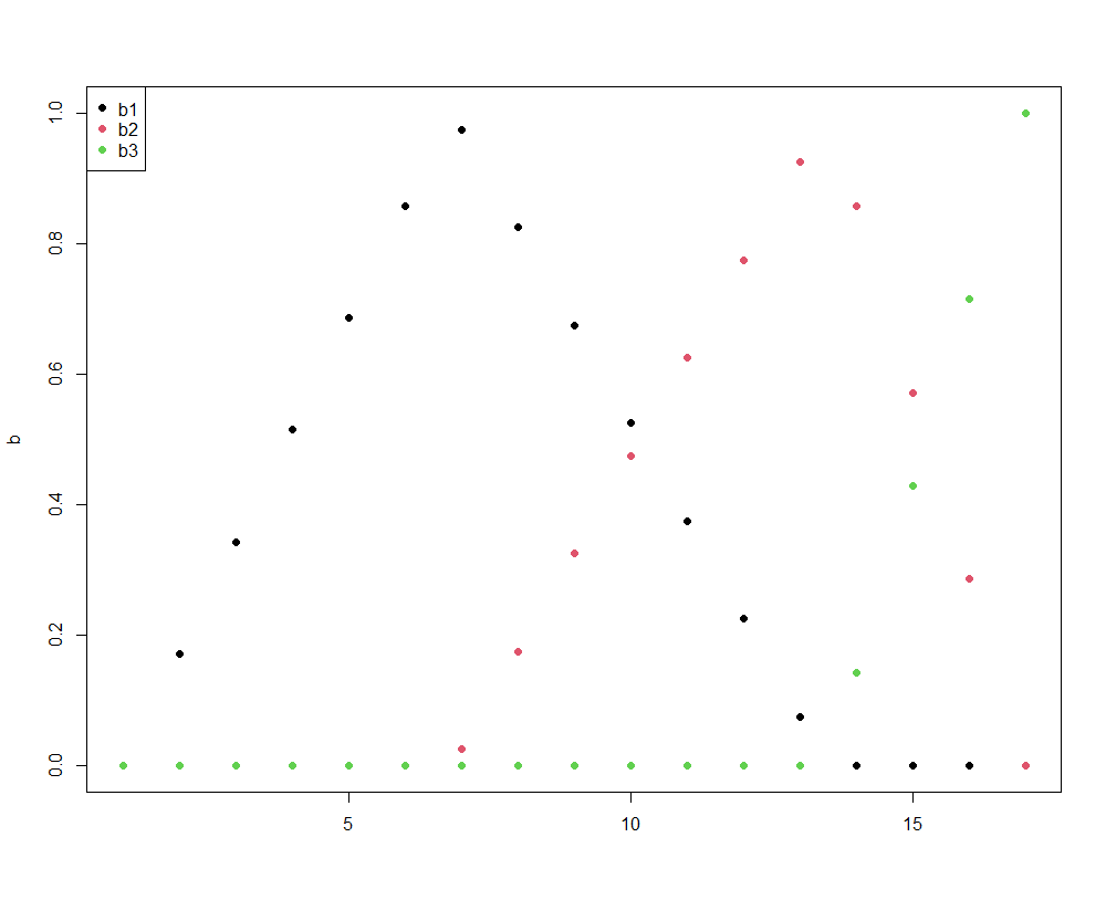
print(b <- trafo(df$power, thres1, thres2))
#              b1        b2        b3
#  [1,] 0.0000000 0.0000000 0.0000000
#  [2,] 0.1714286 0.0000000 0.0000000
#  [3,] 0.3428571 0.0000000 0.0000000
#  [4,] 0.5142857 0.0000000 0.0000000
#  [5,] 0.6857143 0.0000000 0.0000000
#  [6,] 0.8571429 0.0000000 0.0000000
#  [7,] 0.9750000 0.0250000 0.0000000
#  [8,] 0.8250000 0.1750000 0.0000000
#  [9,] 0.6750000 0.3250000 0.0000000
# [10,] 0.5250000 0.4750000 0.0000000
# [11,] 0.3750000 0.6250000 0.0000000
# [12,] 0.2250000 0.7750000 0.0000000
# [13,] 0.0750000 0.9250000 0.0000000
# [14,] 0.0000000 0.8571429 0.1428571
# [15,] 0.0000000 0.5714286 0.4285714
# [16,] 0.0000000 0.2857143 0.7142857
# [17,] 0.0000000 0.0000000 1.0000000

matplot(b, pch = 16)
legend("topleft", legend = c("b1", "b2", "b3"),
       col = 1:3, pch = 16)

plot showing the spline basis

$\endgroup$
7
  • $\begingroup$ thank you for the transformation. But I do not understand the rational of this, nor how to interpret the coefficients when you use such transformation in a regression $\endgroup$
    – denis
    Commented Feb 13 at 7:39
  • 5
    $\begingroup$ Generally, when you use splines, you are not that interested in the coefficients ... $\endgroup$
    – Roland
    Commented Feb 13 at 8:12
  • $\begingroup$ ok, but still it does not answer my question: Why and how this transformation produce the same prediction as my understandable piecewise regression ? What is the rationale of this tranform ? Where does it come from ? How can I reverse it to the slope of each first degree polynomial ? $\endgroup$
    – denis
    Commented Feb 13 at 13:54
  • $\begingroup$ @Roland Could you elaborate on "not that interested in the coefficients"? $\endgroup$
    – rolando2
    Commented Feb 13 at 16:07
  • 1
    $\begingroup$ @Roland I've never heard that distinction made before (not that I am so knowledgeable about splines). I am curious why you make it. I would think that what's good for estimating a main effect of interest would be good for estimating a confounder's effect and vice versa. $\endgroup$
    – rolando2
    Commented Feb 16 at 14:47

Your Answer

By clicking “Post Your Answer”, you agree to our terms of service and acknowledge you have read our privacy policy.

Not the answer you're looking for? Browse other questions tagged or ask your own question.