2
$\begingroup$

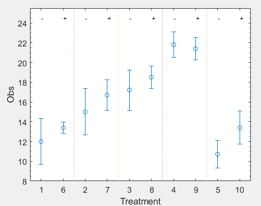
I am puzzled about the result of a 2-way ANOVA analysis. The factors are categorical and non-random and the sum of squares used is constrained type III (the choice of categorical or SS type does not appear to be important to the outcome though). The data consists of 50 measurements, 2 levels in one factor ("catalyst"), 5 in the other ("chemical treatment"), and 5 replicates per treatment. The following error plot illustrates mean +/- std dev for the individual treatments, blocked according to factor #2 (catalyst, with two levels, -/+).

(edit: I substituted a boxplot with an error plot; comments further recommend simply a scatter plot. Note I chose to post a boxplot because this is the default visualization provided by MATLAB ANOVA functions; the documentation of these functions explains the meaning of the lines and symbols which may be somewhat unique).

enter image description here

In the above treatments 1-5 and 6-10 correspond to two levels (-/+) of factor #2 (catalyst) whereas treatments 1-5 differ in factor #1 (chemical treatment, with levels matched by 6-10).

It appears from inspection that factor #1 (chemical treatment) has an effect but the same is hard to say for factor #2 (catalyst).

I ran the analysis in MATLAB as

[p,tbl,model] = anovan(msmnt,{var1,var2},"Model","interaction",'varnames',{'var 1','var 2'}); %Two-Way ANOVA

This is the output table:

Source Sum Sq. d.f. Mean Sq. F Prob>F
factor 1 (chem treatment) 612.97 4 153.242 56.86 0
factor 2 (catalyst) 22.445 1 22.445 8.33 0.0063
factor 1:factor 2 12.53 4 3.132 1.16 0.3418
Error 107.8 40 2.695
Total 755.745 49

There appears to be a significant effect (95% confidence) due to both factors (and no interaction).

I computed some of the ANOVA terms by hand and they (well, my computation) seem correct.

However if you look at the means for each of the two levels of factor #2:

fact#2 (catalyst) level average sample std dev
- 15.35 4.50
+ 16.68 3.34

The error plot (simple inspection) and averages suggest that this is not a significant difference (no effect due to factor #2, catalyst), but the ANOVA table seems to say otherwise.

This conflicting interpretation is confusing. What am I missing in my analysis? Is the ANOVA seeing something I don't?

I suspect the reason is that the within-treatment variances are relatively small. However, if that is true, how do I determine whether the two treatments within individual pairs (eg 1-6, 2-7, etc, differing in presence or absence of catalyst) generate significantly different effects?

$\endgroup$
13
  • 2
    $\begingroup$ This is not a great way to visualize the results because the relatively tiny effect of Factor #2 is swamped by the overall variability. Since Factor #1 has such a strong effect, consider regressing it out and studying how the residuals vary with Factor #2. That will (greatly) magnify the ability of the visualization to detect relatively tiny effects. $\endgroup$
    – whuber
    Commented Apr 8 at 16:08
  • 1
    $\begingroup$ If you are going to use some kind of parallel boxes, I'd line them up in pairs so that your current 1 is next to your current 5, 2 next to 6 and so on. Or, better, you could use some sort of trellis plot. $\endgroup$
    – Peter Flom
    Commented Apr 8 at 16:28
  • 2
    $\begingroup$ There are 49 total degrees of freedom and 10 boxplots. So 5 points per boxplot. This isn't a great choice. See this: How should we do boxplots with small samples?. $\endgroup$
    – dipetkov
    Commented Apr 8 at 18:40
  • 1
    $\begingroup$ And Minimum "recommended" sample size for boxplots? Boxplots for different sample sizes $\endgroup$
    – dipetkov
    Commented Apr 8 at 18:53
  • 1
    $\begingroup$ Why don't you plot the actual data points? You have 50 points and you can make an effective plot showing all of them. (That's the advice in the CV threads I linked to. If you're not sure how, that's a new question.) It seems that in your current viz you calculate standard errors separately for each treatment but that's not how anova models the data. $\endgroup$
    – dipetkov
    Commented Apr 9 at 9:22

1 Answer 1

1
$\begingroup$

When you take the simple means of the DV by factor level, you are not controlling for the other variable. With ANOVA, you are. You would have to look at the means of the two levels of that factor for each of the five levels of the other. (It would have made this easier to write if you had told us what these factors are).

This is like comparing 1 to 5, 2 to 6, 3 to 7, and so on in the plot. Also, that's not a usual boxplot. I did a very little bit of Googling and did not find one like it. It's a little like a violin plot. But what are the extra lines?

$\endgroup$
14
  • $\begingroup$ Matlab details boxplots here (see the "more about" section). $\endgroup$
    – Buck Thorn
    Commented Apr 8 at 16:15
  • $\begingroup$ "It would have made this easier to write if you had told us what these factors are". For factor#1 there are 5 levels (eg treatments 1-5 differ in this factor) , it is categorical. The boxplot shows the means +/- sd (and percentiles) for each treatment (corresponding to combination of factors 1 and 2): there are 2x5 possible treatments. $\endgroup$
    – Buck Thorn
    Commented Apr 8 at 16:22
  • 1
    $\begingroup$ I am confident Peter is not asking what a boxplot is. One of the (many) problems with the plots in the question is that they do not clearly reveal the two-factor structure of the analysis (nor do they help at all with the interaction). The use of confidence bands for boxplots that represent only 5 values each is unnecessary and visually confusing, too. (Typically there are more graphical elements in each box then there are data behind it!) You could do much better plotting the data themselves on dot plots. $\endgroup$
    – whuber
    Commented Apr 8 at 16:22
  • 1
    $\begingroup$ Thanks for your answer. Upon review it seems showing boxplots was a mistake. I picked this somewhat out of convenience (it is the default display method in Matlab when performing ANOVA). A scatter plot would have been better as whuber and dipetkov pointed out. Your answer though does answer my actual question, and whuber pointed out why I missed the obvious. Factor #1 has a strong effect and #2 weak (I suspected none but the ANOVA identified one). $\endgroup$
    – Buck Thorn
    Commented Apr 10 at 7:56
  • 1
    $\begingroup$ @whuber To be fair I was stumbling a bit in the dark. The MATLAB documentation is not great. In general the statistics package hides the computations being performed (R code is not much better but the documentation is; I realize a more advanced textbook might include relevant details). This also got wrapped up in discussion of plots (which was useful). The small effect of factor 2 is obfuscated by the presentation, as this answer points out. A comment suggested I read up on contrasts. I edited to clarify the q: how to determine significance of fact #2, including within individual pairs. $\endgroup$
    – Buck Thorn
    Commented Apr 11 at 8:44

Your Answer

By clicking “Post Your Answer”, you agree to our terms of service and acknowledge you have read our privacy policy.

Not the answer you're looking for? Browse other questions tagged or ask your own question.