Detect rare high-value measurements in a series of measurements

Question

We do a measurement on 1000 samples to detect if a chemical element A is present, and for each measurement, two cases can happen :

• the element A is not present, and the values we get are a "background noise", with a gaussian distribution $N(100, 15)$.

• the element A is present, and then we get values around $120$.

Given a list of 1000 measurements [101.1, 98.2, 123.12, ..., 125.5], how can we conclude with a given confidence %, that, the element A has been found at least once, or at least k times, etc. ?

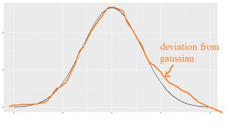
Intuitively, we can look at the histogram, and see if it deviates or not from a gaussian curve. How can we turn this into a quantitative solution?

Are there solutions where I subtract the density of N(100, 15) (=the black curve) from the normalized histogram of the sample (=the orange curve), and see if the difference can highlight a population:

?

Answer 1

The natural way to model this is as a mixture of two Normal distributions. Proportion $\pi$ of the data comes from distribution 1, which has a mean of 100, a standard deviation of 15. Proportion $1 - \pi$ comes from distribution 2, which has a mean of 120, and an unknown standard deviation (unless you're able to provide one). You're primarily interested in estimating $1 - \pi$.

There are lots of tools for estimating Gaussian mixture models, but most won't quantify uncertainty in the proportions, as far as I know. I would therefore reach for Bayesian tools like Stan here. Here's a very rough implementation of this idea, based on an example from the rstan documentation. If anyone wants to edit this answer to provide more explanation, please feel free.

library(rstan)
# Simulate data
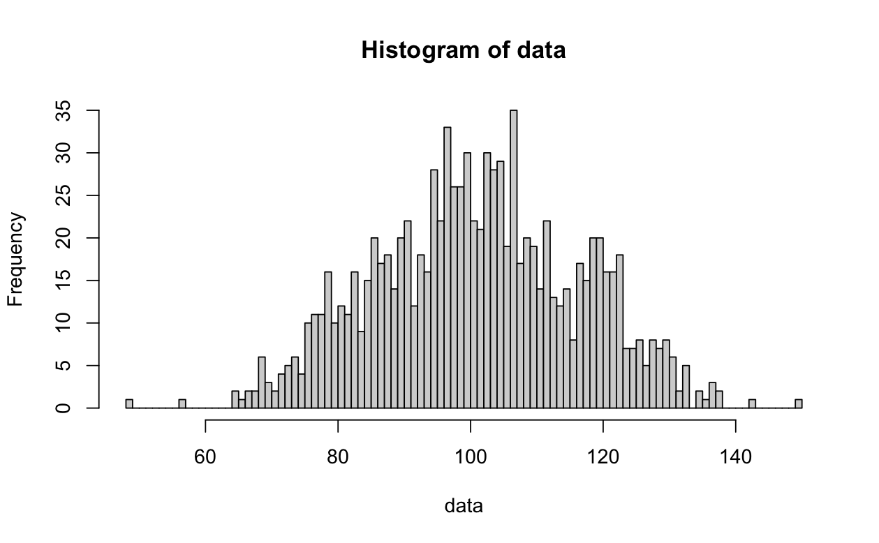
n = 1000
n_k = 50
data = c(
  rnorm(1000 - n_k, 100, 15),
  rnorm(n_k, 120, 2)
)
hist(data, breaks=101)

Stan model

data {
  int N;
  vector[N] y;
}
parameters {
  ordered[2] mu;
  vector<lower = 0>[2] sigma;
  // Here, Theta[1] = pi, Theta[2] = 1-pi
  simplex[2] Theta;
}
model {
  vector[2] contributions;
  // priors
  mu[1] ~ normal(100, .1);
  sigma[1] ~ normal(15, .1);
  mu[2] ~ normal(120, .1);
  sigma[2] ~ cauchy(0, 1);
  Theta ~ dirichlet(rep_vector(2.0, 2));
  
  // likelihood
  for(i in 1:N) {
    for(k in 1:2) {
      contributions[k] = log(Theta[k]) + normal_lpdf(y[i] | mu[k], sigma[k]);
    }
    target += log_sum_exp(contributions);
  }
}

stan_data = list(
  N = length(data),
  y = data
)
stan_result = rstan::sampling(mm_stan_model, data=stan_data, iter=2000)
stan_result
# Inference for Stan model: stan-c893ebbe0d5.
# 4 chains, each with iter=2000; warmup=1000; thin=1; 
# post-warmup draws per chain=1000, total post-warmup draws=4000.
# 
#              mean se_mean   sd     2.5%      25%      50%      75%    97.5% n_eff Rhat
# mu[1]      100.00    0.00 0.10    99.80    99.94   100.00   100.07   100.20  3301 1.00
# mu[2]      120.01    0.00 0.10   119.81   119.94   120.01   120.08   120.21  3289 1.00
# sigma[1]    15.01    0.00 0.10    14.82    14.95    15.01    15.08    15.20  4030 1.00
# sigma[2]     1.97    0.03 0.75     1.15     1.56     1.82     2.14     4.03   457 1.00
# Theta[1]     0.95    0.00 0.01     0.93     0.94     0.95     0.96     0.97   910 1.00
# Theta[2]     0.05    0.00 0.01     0.03     0.04     0.05     0.06     0.07   910 1.00
# lp__     -4145.98    0.06 1.71 -4150.22 -4146.90 -4145.62 -4144.69 -4143.77   795 1.01
# 
# Samples were drawn using NUTS(diag_e) at Mon Apr 22 13:49:35 2024.
# For each parameter, n_eff is a crude measure of effective sample size,
# and Rhat is the potential scale reduction factor on split chains (at 
# convergence, Rhat=1).

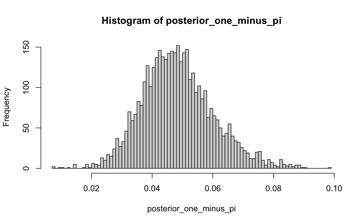
posterior_samples = extract(stan_result)
posterior_one_minus_pi = posterior_samples$`Theta`[,2]
hist(posterior_one_minus_pi, breaks=101) # Proportion of values that are outliers

Update

There's actually a simpler approach here, if you are willing to assume the means and standard deviations of the two distributions, but I don't have time to go into it.

Answer 2

Answering questions such as element A has been found at least once, or at least k times, etc. is not simple. It's easier to answer questions pertaining to the whole sample rather than individual units.

What you could do is compare your obtained distribution with a reference distribution having mu and sigma equal to 100 and 15 (assuming you know these values and they are true) by using the Kolmogorov-Smirnov test. You could also use a test for checking whether your distribution is "normal" (which it wouldn't be if element A is present and you would have a bimodal distribution) by using the Shapiro-Wilk test.

You could also simply compare the mean to 100 using a (one sided?) t-test.