8
$\begingroup$

I would be interested in a method to find an appropriate Lambda parameter for the Box-Cox transformation based on only the skewness and the kurtosis of a given sample.

I.e, if the skewness and kurtosis indicate that the data might be normal (i.e., skewness of 0 and kurtosis of 3) the method should choose a Lambda of 1. If the skewness and kurtosis deviate from these values, the Lambda should be chosen such that the deviation are corrected as well as possible.

I was not able to find prior work that proposes such a method. Is there someone who might be able to help me out in this regard?

$\endgroup$
2
  • $\begingroup$ Do you happen to have data examples you can share or at least visualize the density / histogram / ecdf ? That would help guide some of the options you have (if data is clearly not even unimodal and / or negative valued it would lead to different suggestions than if it's "nice" unimodal and/or positive values ) $\endgroup$ Commented Jun 2 at 21:23
  • $\begingroup$ @GeorgM.Goerg It's often understandable if people are more interested in answering a different question, but equally the question here is not at all how do I choose a transformation for my data. It's nicely specific -- how do I get from skewness and kurtosis to choosing a good transformation -- and the answers vary in their reasons for saying that such a goal is not at all a good idea. $\endgroup$
    – Nick Cox
    Commented Jun 4 at 12:22

4 Answers 4

16
$\begingroup$

There are several reasons why you have not found any such procedure. Some are very simple and may seem utterly obvious, but that doesn't make them less compelling.

  1. Skewness and kurtosis in the sense of moment-based measures are just one possible choice of measures of "skewness" or "kurtosis" in some Platonic sense. To be less cryptic, there are vague concepts of asymmetry and tail weight of distributions that can be made precise and quantified in many different ways. Moment-based measures can be, for example, over-sensitive to outliers and they pose more subtle problems in being limited as functions of sample size, so that a sample may not be able to exhibit the skewness and kurtosis of its parent family.

  2. Skewness and kurtosis can be calculated for counted or measured variables regardless of whether values are negative, zero or positive, but the Box-Cox power family in its simplest form usually presupposes positive or at least non-negative values.

  3. Similarly skewness and kurtosis can be calculated for bounded variables -- such as those observed on, or mappable to, $(0, 1)$ or $[0, 1]$ -- but if transformations make sense for the latter they are usually of different form, e.g. logit rather than logarithm. An even more extreme case is that of $(0, 1)$ indicator variables which often exhibit extreme skewness but which cannot be transformed in any useful way.

  4. Such a formulation places even more stress in the wrong place than do naive or over-simplified treatments of Box-Cox by arguing or implying that getting closer to normal marginal distributions is the main deal. On the contrary, even for regression-type models it's at most conditional distributions being close to normal that is some kind of ideal. More generally, what is most valuable about a transformation -- if it is valuable at all -- is likely to be getting closer to (in rough order of importance) additivity, linearity, homoscedasticity and symmetry -- with normality as a special case of the latter being least important of all ideal conditions (often unfortunately stated as assumptions).

  5. Transformations divide the statistical world, and this community too. There are leading members here who never saw a transformation they didn't dislike -- and leading members too who are very positive about transformations being often useful when carefully chosen (above all for visualizing data or results). But there is perhaps slowly and steadily growing recognition that (in jargon introduced with generalized linear models) using link functions other than identity is in many ways a deeper and more helpful way to deal with awkward (e.g. skewed or long-tailed) outcomes. A canonical example here is Poisson regression which does not entail transforming an outcome but respects the scale of the outcome by estimating positive mean functions. Transformations can still make sense for predictors.

  6. I take from the Box and Cox analysis two main ideas, neither quite original even at the time, but both pushed well in their paper: (a) the most common transformations aren't a ragbag of small mathematical tricks but form a family (b) the data themselves can indicate a transformation that may be appropriate, or (just as valuable) that a range of transformations may be appropriate. It's notable that their empirical examples are used to motivate logarithmic and reciprocal transformations that would have seemed sensible to experienced practitioners any way. What I think is contrary to the spirit of their paper is any idea that you can and should automate choice of transformation or that there are calculations that will indicate that power 0.123 or whatever is the transformation to use. Their intent aside, in 60 years since their paper (1964), other methods have emerged strongly that offer other solutions in different ways given awkward distributions.

  7. When faced with the same variables in different groups or in different datasets, it is usually more valuable to treat them consistently than to optimize in terms of what seems best to suit particular skewness or kurtosis. Typically a scale -- in terms of either a transformation or a link function -- should be chosen consistently on substantive or scientific grounds (e.g. physical, biological, economic). Most often that means working on logarithmic scale.

In short, this procedure doesn't obviously exist -- and isn't even a good idea in principle -- because you need to know much more than skewness and kurtosis to know whether a transformation is a good idea at all, let alone which transformation(s) are worth trying, principally

  • what model is envisaged

  • what variables are candidates for inclusion in a model

  • what role does any variable play, outcome or predictor

  • what is the range of values observed in practice

  • what is the range of values possible in principle

$\endgroup$
9
  • 4
    $\begingroup$ Disclaimer: Although the term Box-Cox is personally appealing, my family name is otherwise irrelevant to the issues. $\endgroup$
    – Nick Cox
    Commented May 24 at 15:45
  • 2
    $\begingroup$ Great answer, but (unless I managed to miss it, which I might have), it doesn't seem to address the issue that a location-shift will leave skewness and kurtosis unchanged but (assuming it remains within the region where such transformations work) will certainly change the impact of the transformation. e.g. if X1 ~ exp(1) and X2=X1+5, then skew(X1) = skew(X2) and kurt(X1)=kurt(X2) but a transformation that works quite well for X1 will not work at all for X2. Consequently skewness and kurtosis cannot of themselves ever hope to be sufficient as a way to identify a suitable power transformation. $\endgroup$
    – Glen_b
    Commented May 24 at 23:26
  • 2
    $\begingroup$ In the case of the exponential, $X_1^p$ where $p\approx 1/3.6$ works quite well as a symmetrizing transform, but $X_2^p$ is almost useless, in spite of their identical skewness and kurtosis. As Nick points out, transformation changes multiple things; usually the distribution shape is less important than things like linearity or near-constant variance. ... (Nick, if you have any interest in including this point in your answer, please feel free. If not, that's fine too. If you did already and I did miss it, my apologies.) $\endgroup$
    – Glen_b
    Commented May 24 at 23:29
  • 1
    $\begingroup$ @Glen_b Your excellent points would go best as an extra answer. There may be counter-examples, but my if zero has a clear physical, biological or other meaning (e.g. zero mass or income or children) there is no obvious gain from shifting the origin, whereas if zero is an arbitrary choice (Celsius or Fahrenheit temperature) almost no transformation is helpful any way. This could be phrased in terms of the distinction between ratio and interval scale measurements. My closing comments that you need to know more about a variable than just skewness and kurtosis could be expanded in this way. $\endgroup$
    – Nick Cox
    Commented May 25 at 0:04
  • 1
    $\begingroup$ Thanks, I'll think about an answer. I wasn't proposing that anyone would be actually shifting the origin of their data in practice (though that certainly happens now and then); the underlying point was simply to show that it was a trivial matter to construct two distinct variables with identical skewness and kurtosis but very different response to transformation to show that those measures are no help on their own; a shift is the easy way to get to examples. Indeed that might also be worth showing in a second way (i.e. to show that you can get the same issue without location shift). $\endgroup$
    – Glen_b
    Commented May 25 at 6:39
8
$\begingroup$

I'm more of someone @nick-cox terms "I never met a transformation I didn't dislike" kind of statistician. It is ironic that we seek transformations that fit the data, yet "fit the data" means agreement with the empirical cumulative distribution function (ECDF). ECDF-guided model selection will inherit the variance of ECDF so provides little advantage over just using the ECDF. This is what ordinal semiparametric regression models do, as described here. You do not need to worry about the transformation of $Y$. Ordinal regression takes into account transformation uncertainty, unlike trial-and-error procedures which result in too-narrow confidence bands by not taking model uncertainty into account. These are reasons the Cox proportional hazards model is so popular, and why the proportional odds model is rapidly gaining in popularity.

In addition to handling extreme skewness and kurtosis, ordinal models handle bimodality, detection limits, and floor and ceiling effects.

$\endgroup$
6
  • 2
    $\begingroup$ Transformation is one of the worst taught and least well understood parts of statistics. One reason why: you need expertise and experience to judge whether a transformation helps. Like many others, since high school I've seen many examples where logarithms in particular make behaviour easier to see and to model -- but equally there are many examples where transformation doesn't help or there is a better idea. The chicken-and-egg problem with your favourite model here is that more people would try it if they saw examples all over their own literature. You're doing your best to evangelise... $\endgroup$
    – Nick Cox
    Commented May 26 at 11:15
  • 1
    $\begingroup$ Well put. Another side of this is that many economists feel you should model on the original scale because it provides the mean directly in a linear model. This is wrong on so many levels: (1) you can estimate the mean from a transformed model using the smearing estimator, (2) you can estimate the mean fairly directly from a model that doesn’t assuming anything about the transformation, and (3) estimating coefficients when you should have transformed Y will result in bad coefficients that give wrong predictions for everyone though right on the average. $\endgroup$ Commented May 26 at 11:55
  • $\begingroup$ Well, I am not an economist, so don't feel criticised there. But often something like a generalized linear model does give you the best of both worlds. $\endgroup$
    – Nick Cox
    Commented May 26 at 12:01
  • $\begingroup$ If you are really correct about the assumed transformation. $\endgroup$ Commented May 26 at 12:09
  • $\begingroup$ If I use a log link or a logit link, I am presuming much more about a sensible functional form than about any marginal or conditional distribution -- and I have flexibility about what family I specify. That stance doesn't rule out being willing also to entertain models that are one way or another just smoothing the data. $\endgroup$
    – Nick Cox
    Commented May 26 at 12:23
8
$\begingroup$

The answer by @Nick Cox is very thorough and informative and I believe you should accept it.

Although Nick is correct that such a procedure does not exist, I wanted to provide you with some tools that may be at least partially useful for you. The short of it is, you can try to find a distribution (or several) which is consistent with the data you have (even if that is limited the the skew and kurtosis). After you have identified a reasonable distribution, you may be able to find a custom transformation that works for you. For example, if an Exponential distribution seems to provide a reasonable fit for $X$, then the transformation $U = -\log X$ will be approximately uniform on $(0, 1)$, which can be easily transformed to a logistic or Gaussian distribution (if you really really need this).


Cullen-Frey Plot

The R package fitdistrplus provides a nice implementation of the Cullen-Frey plot, which attempts to identify a distribution based only on the kurtosis and the square of the skewness.

# Simulate some data
n <- 500
y <- rgamma(n, 3, 1.5) + rlnorm(n, 1, 0.5)

#install.packages("fitdistrplus")
library(fitdistrplus)
descdist(y)
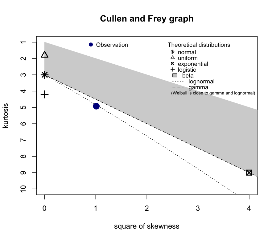
Cullen-frey plot

This figure suggests that a lognormal distribution may be roughly consistent with these data. This in-turn suggests that the transformation $\log X$ will yield data which may be approximately Gaussian.


The Normal-Wald Triangle Plot

The Normal-Wald distribution is a highly flexible 3-parameter distribution which can capture both left and right skew as well as a wide variety of tail behaviors.

The Normal-Wald triangle plot is a useful tool for assessing the behavior of a data-set, using steepness (akin to kurtosis) and asymmetry (akin to skewness). See this paper or Sections 3.4.1 and SM6 of this paper for details.

library(devtools)
#devtools::install_github("knrumsey/GBASS")
library(GBASS)
X <- matrix(rep(1, n), ncol=1)
fit <- nwbass2(X, y,
               m_gamma=-1.4, s_gamma=82,
               m_beta=0, s_beta=0.5)
nw_triangle(fit, bg='orange', pch=21, cex=1.5, details=TRUE)

# Alternatively, gain point estimates only using the moments
# Fix location = 0, scale = 1
skew <- mean(((y-mean(y))/sd(y))^3) # sample skewness
kurt <- mean(((y-mean(y))/sd(y))^4) # sample kurtosis
stats <- c(NA, NA, skew, kurt)
nw_est_mom(stats=stats, mu=0, delta=1, triangle=TRUE)
## returns: (0.3089, 0.6740)

# With an additional moment, we can estimate the scale param as well
stats <- c(NA, var(y), skew, kurt)
nw_est_mom(stats=stats, mu=0, triangle=TRUE)
## returns: (0.4437, 0.7399)
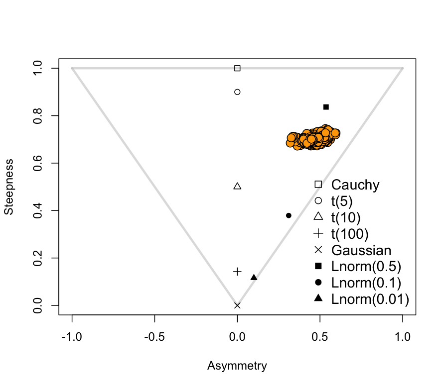
NW Triangle

As with Cullen-Frey, this figure indicates that a log-normal distribution may be consistent with these data.

$\endgroup$
7
  • 1
    $\begingroup$ (+1) Very helpful. Rhind, A. 1909. Tables to Facilitate the Computation of the Probable Errors of the Chief Constants of Skew Frequency Distributions. )Biometrika_ 7: 127–147. doi.org/10.2307/2345367 and 1910. Additional Tables and Diagram for the Determination of the Errors of Type of Frequency Distributions. Second Paper. Biometrika 7: 386–397. doi.org/10.2307/2345391 gave plots of skewness and kurtosis. Rhind worked with Karl Pearson. $\endgroup$
    – Nick Cox
    Commented May 25 at 8:00
  • $\begingroup$ One of the simplest examples in this territory is the lognormal, but your second diagram in particular implies that logarithm may be the ideal transformation for a range of distribution shapes. So, like all such aids, it needs to be used carefully and circumspectly, and I imagine that you would underline that emphatically, but it's evidence against the very naive hope that shape measures alone give good guidance on whether and how to transform. $\endgroup$
    – Nick Cox
    Commented May 26 at 10:32
  • 1
    $\begingroup$ This is indeed a very helpful answer, which puts me on the right track in a practical sense. Nevertheless, I will follow your suggestion and accept the answer by Nick Cox, because he discussed the problem on a more fundamental level. $\endgroup$
    – Hiro
    Commented May 27 at 11:24
  • 1
    $\begingroup$ I had some time to look at the links. It may not be obvious to others, so I will flag that in the second diagram, asymmetry and steepness are names given to parameters estimated from the data in the course of estimating a normal-Wald distribution. They aren't independently derived as descriptive statistics. $\endgroup$
    – Nick Cox
    Commented May 28 at 15:04
  • 1
    $\begingroup$ @NickCox Thanks for pointing that out and clarifying for future readers. Of course, through a Method of Moments type approach, we can define "steepness" and "asymmetry" in terms of the sample moments (regardless of distribution). If we only have two moments (e.g., skew and kurtosis), then we need to fix the scale parameter at a reasonable value. We can improve our estimation by including a third moment (e.g., the variance). I have edited the answer include R code for both cases. $\endgroup$
    – knrumsey
    Commented May 28 at 19:16
7
$\begingroup$

Unless you impose some pretty restrictive conditions, using skewness and kurtosis as a basis to choose a transformation is not useful.

Indeed a number of textbooks used in some particular application areas contain prescriptions about how much skewness suggest either an identity, a square root or a log transformation (some may suggest some other transformations in addition or in place of some of these). As we will see below, such advice based on standardized moments is clearly misplaced in general; indeed in some cases such advice may well make things worse.

There's multiple ways to see that distributions with the same skewness (or even skewness and kurtosis together) may need very different transformations. Consequently skewness and kurtosis cannot of themselves ever hope to be sufficient as a way to identify a suitable power transformation.

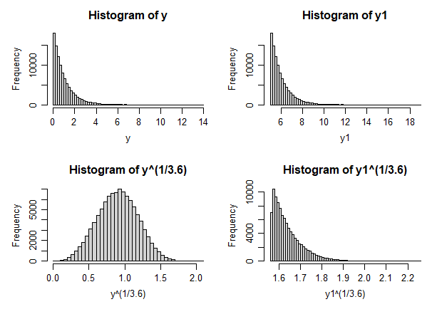
  1. A location-shift will leave skewness and kurtosis unchanged but (assuming it remains within the region where such transformations work) will certainly change the impact of the transformation. e.g. if $X_1 \sim \text{Exp}(1)$ and $X_2=X_1+5$, then $\text{skew}(X_1) = \text{skew}(X_2)$ and $\text{kurt}(X_1)=\text{kurt}(X_2)$ but a transformation that works quite well for $X_1$ will not work at all for $X_2$.

    In the case of the exponential, $X_1^{p}$ where $p≈1/3.6$ works quite well as a symmetrizing transform (it's not very far from a monotonic transformation to exact normality and the choice of values near to the reciprocal of $3.6$ can be guessed from the connection to the Weibull), but $X_2^{p}$ is almost useless, in spite of their identical skewness and kurtosis.

    Two distributions with identical shape and so identical skewness and kurtosis but where different transformations required

    Here y corresponds to $X_1$ above and y1 corresponds to $X_2$.

    To be clear, I am not proposing that anyone should be actually shifting the origin of their data as I did here. The aim is just to show by the simplest means that we can have two distinct variables with identical skewness and kurtosis but very different response to transformation. Indeed in this example, all the higher standardized moments would be equal as well, so choosing still more such standardized-moment-based coefficients will not help; indeed anything that simply considers shape alone cannot suffice, even if you perfectly describe the shape, since the exponential and the shifted exponential have identical shape.

  2. At the same time, exactly the same transformation may be suitable for a wide range of different values of skewness and kurtosis. For example, every lognormal distribution has the same symmetrizing transformation (the log, naturally), but skewness and kurtosis are both functions of the shape parameter $\sigma$. Indeed the skewness of a lognormal can be anything from as near to $0$ as you wish to extremely skewed (albeit still finite). Similarly the kurtosis can be anything from very close to that for a normal to extremely large. But the same transformation (the log) is the correct choice for all of them. So again, we are left to conclude that the skewness and kurtosis cannot necessarily help us choose the correct transformation in general.

    The lognormal is not the only distribution family with this property, it's just a simple example where the 'correct' transformation to use is not a matter for debate.

  3. It's perfectly possible to construct pairs of distributions where power transformations make sense for both but where we have a pair of distributions where the weaker transformation goes with the more skewed and more kurtotic distribution.

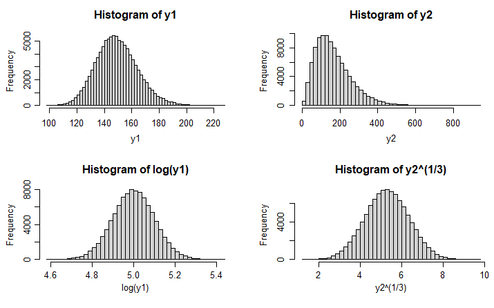
    An example is provided by lognormal and gamma distributions. As we saw in point 2, the lognormal may be anywhere from quite near to the normal (only very mildly right skew and only very mildly more kurtotic than the normal) to very skewed and kurtotic, but we can choose a gamma distribution that's more skew and with larger kurtosis.

    Except for small values of the gamma shape parameter, the best choice of Box-Cox transformation will be close to the cube root (the Wilson-Hilferty transformation). For smaller values, a slightly stronger power transformation may do better (e.g. as we saw above, when the shape is $1$, the $3.6$th root is a good choice and for slightly smaller shape parameters the fourth root may be a reasonable choice), but for each of them the log transformation will make it left-skewed. The log is "too strong" for the gamma even when it's quite skewed.

    Lognormal (chosen to be very mildly skew) and gamma distributions (chosen to be more skew) and suitable choices of Box Cox transformations for each (log and cube root)

    Here we have a lognormal on the left and a gamma on the right. The gamma is more skewed and kurtotic but the correct transformation for the lognormal would be too much for the gamma. As we see, the more skewed gamma only requires a cube root transformation.

    Here the $\sigma$ parameter of the lognormal was $0.1$, while the shape parameter of the gamma was $3$, resulting in greater skewness and kurtosis for the gamma, but nevertheless the gamma required a weaker transformation to get close to normality.

    In another of my answers (which I could not locate just now) I looked at a distribution family for which the square root was a good choice of power transformation. Nevertheless, it would be possible to choose a member of such a family that was more skewed than some gamma and which was in turn more skewed than some lognormal, where the the weaker power transformations would go with the stronger skewness and the strongest transformation would go with the weaker skewness.

  4. We can readily find population distributions which are quite distinctly non-normal but which have the same skewness and kurtosis as the normal (there are both discrete and continuous examples as well as examples which are neither). Naturally a skewness-and-kurtosis-based rule looking at the whole distribution (or even very large samples) would not transform these distributions at all, leaving us with the distinctly-non-normal distributions we began with. We can widen the class of allowed transformations and (assuming our example was one of the continuous possibilities) identify exact transformations to normality, but these perfect transformations could not be indicated by the skewness and kurtosis.

Many other examples may be produced which clearly show that skewness and kurtosis are not of themselves a good guide to choice of transformation.

$\endgroup$
1
  • $\begingroup$ I really like your clear explanations and concrete examples! $\endgroup$ Commented Jun 3 at 19:27

Your Answer

By clicking “Post Your Answer”, you agree to our terms of service and acknowledge you have read our privacy policy.

Not the answer you're looking for? Browse other questions tagged or ask your own question.