There are a bunch of ways.
Two reasonably popular ways are the Brier score and the log loss. The Brier score is square loss, the same as mean squared error: $\text{Brier}\left(e, p\right) = \dfrac{1}{N}\overset{N}{\underset{i = 1}{\sum}}\left(y_i - e_i\right)^2$. Brier score can be normalized by comparing to predicting the mean of $y$ every time, what UCLA calls Efron's pseudo $R^2$.
$$
R^2_{\text{Efron}} = 1 - \left(\dfrac{
\overset{N}{\underset{i = 1}{\sum}}\left(y_i - e_i\right)^2
}{
\dfrac{1}{N}\overset{N}{\underset{i = 1}{\sum}}\left(y_i - \bar y\right)^2
}\right)
$$
Brier score is a metric in the sense of a metric space.
The log loss is the canonical loss function in "classification" problems and sometimes goes by the names "crossentropy" or "negative log likelihood", the latter of which alludes to the relationship with maximum likelihood estimation with a Binomial likelihood. Log loss has a formula that is a bit nastier than Brier score but isn't all that bad.
$$
\text{LogLoss}\left(e, p\right) = -\dfrac{1}{N}\overset{N}{\underset{i = 1}{\sum}}\left[
y_i\log(e_i) + (1 - y_i)\log(1 - e_i)
\right]
$$
Log loss can be normalized by comparing to predicting the mean of $y$ every time, what UCLA calls McFadden's pseudo $R^2$.
$$
R^2_{\text{McFadden}} = 1 - \left(\dfrac{
\overset{N}{\underset{i = 1}{\sum}}\left[
y_i\log(e_i) + (1 - y_i)\log(1 - e_i)
\right]
}{
\overset{N}{\underset{i = 1}{\sum}}\left[
y_i\log(\bar y) + (1 - y_i)\log(1 - \bar y)
\right]
}\right)
$$
Log loss is not a metric in the sense of a metric space (not commutative, maybe other axioms violated), but it seems to be acceptable slang to refer to any measure of performance as a performance metric.
That UCLA page mentions a number of other possible measures of performance. An advantage of Brier score and log loss is that they are so-called strictly proper scoring-rules that are uniquely optimized in expectation by the "correct" probabilities. The advantages of working with strictly proper scoring rules are discussed extensively on Cross Validated, with this question serving as a good introduction that can send you down the rabbit hole.
Normalizing as the Efron and McFadden pseudo $R^2$ is totally aligned with how Gneiting and Resin (2023) develop the $R^*$ of their equation (32) that they call a universal coefficient of determination.
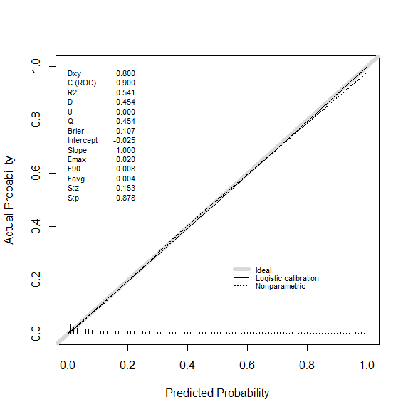
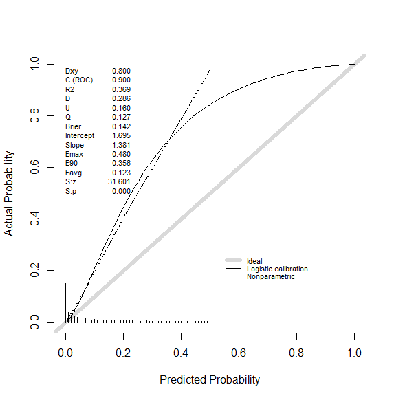
Another useful assessment is of the calibration, if claimed probabilities really correspond to event occurrence probabilities. The Scikit-learn documentation has a nice page on this, with the package containing some functions to perform such analysis. For R users, rms::val.prob could be of value. For instance, in the below examples, the first shows good calibration in that the claimed probabilities in p1 correspond with the reality of event occurrence. However, the second shows poor calibration, with the claimed probabilities in p2 not corresponding with the reality of event occurrence (e.g., claimed probability of $0.4$ corresponds with a real event occurrence probability of around $0.7$).


library(rms)
set.seed(2024)
N <- 10000
p1 <- rbeta(N, 1/3, 1)
y <- rbinom(N, 1, p1)
rms::val.prob(p1, y)
p2 <- p1/2
rms::val.prob(p2, y)
REFERENCE
Gneiting, Tilmann, and Johannes Resin. "Regression diagnostics meets forecast evaluation: Conditional calibration, reliability diagrams, and coefficient of determination." Electronic Journal of Statistics 17.2 (2023): 3226-3286.


