Errors on cubic fits are relative to the order of magnitude of the y-data, not fit quality

Question

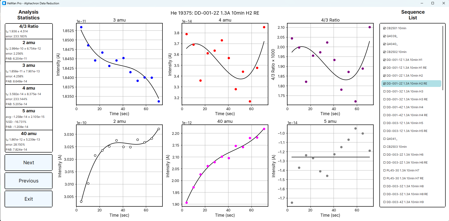
I am writing some mass spec data reduction software (specifically, residual gas analysis mass spectrometry). I recently implemented a cubic fitting algorithm as an optional feature, however, some of the errors on the t=0 intercepts I'm seeing relate more to the order of magnitude of the data rather than the goodness of fit. Here are some examples:

Before digging into these examples, I suggest that you ignore the 4/3 Ratio and 5 amu data; the 4/3 Ratio is calculated from 3 amu and 4 amu data, and the 5 amu data are the baseline (no gaseous species at 5 amu) so we always use an average instead of applying a linear/curve fit.

The errors are:

2 amu: 3%

3 amu: 6%

4 amu: 218%

40 amu: 67%

Basic observations:

1. 40 amu forms a very clear trend and should have the lowest error of any of these fits.
2. 3 amu barely forms a clearer trend than 4 amu, if at all.

I would therefore expect the error on the 3 and 4 amu fits to be relatively similar, maybe a little higher for 4 amu, and the 40 amu error to be very low; what I'm seeing, however, is that, because 4 amu is down around 3e-14 A, and 40 amu is down around 6E-13 A, these signals end up with relatively higher errors than higher signals.

Because the 2 amu signal (pesky ol' hydrogen) is the strongest and clearest of all, it ends up with the lowest error.

Here's another example:

The errors on the intercepts are clearly more related to the order of magnitude of the y-data than the actual fit.

Here is the cubic fitting function:

def cubic(x, a, b, c, d):
    return a * x**3 + b * x**2 + c * x + d

def cubic_curve_fit(x,y):
    popt, pcov = curve_fit(cubic, x, y)
    
    fitted_x = np.linspace(min(x), max(x), 100)
    fitted_y = cubic(fitted_x, *popt)
    intercept = cubic(0, *popt)
    
    # calculate the standard error of the intercept
    residuals          = y - cubic(x, *popt)
    residual_variance  = np.sum(residuals ** 2) / (len(x) - 4)
    intercept_variance = residual_variance * np.sum(x ** 2) / len(x)
    intercept_stderror = np.sqrt(intercept_variance)
    
    return [fitted_x, fitted_y], intercept, intercept_stderror

And here are the sample data for the two examples shown:

Example 1:

He 19371    CB2502 10min    2022-06-29T08:50:40 
time_sec    2 amu   3 amu   4 amu   5 amu   40 amu
4.589   2.499294E-10    1.883895E-11    3.761834E-14    -1.506364E-14   5.055386E-13
10.589  2.506302E-10    1.885923E-11    3.718189E-14    -1.425650E-14   5.364334E-13
16.789  2.510879E-10    1.886623E-11    3.406583E-14    -1.196330E-14   5.470421E-13
22.789  2.516341E-10    1.879266E-11    3.178908E-14    -9.997409E-15   5.628271E-13
28.889  2.518049E-10    1.881801E-11    3.205416E-14    -1.030216E-14   5.570411E-13
34.989  2.515727E-10    1.880201E-11    3.486602E-14    -1.284306E-14   5.819271E-13
41.089  2.518113E-10    1.874990E-11    3.815993E-14    -1.486189E-14   5.917647E-13
47.189  2.520151E-10    1.876996E-11    3.482708E-14    -1.231443E-14   6.122757E-13
53.289  2.521316E-10    1.874753E-11    3.708621E-14    -1.313210E-14   6.292820E-13
59.289  2.525987E-10    1.880525E-11    3.839327E-14    -1.173513E-14   6.401169E-13
65.389  2.526217E-10    1.875623E-11    3.478337E-14    -1.153751E-14   6.546364E-13
71.489  2.528286E-10    1.880495E-11    3.933710E-14    -1.402713E-14   6.577292E-13

Example 2:

He 19375    DD-001-2Z 1.3A 10min H2 RE  2022-06-29T10:35:05
time_sec    2 amu   3 amu   4 amu   5 amu   40 amu
4.015   3.003075E-10    1.853406E-11    3.788137E-14    -1.749695E-14   1.906308E-12
10.115  3.010267E-10    1.848526E-11    3.689935E-14    -1.372115E-14   1.971391E-12
16.115  3.021516E-10    1.844551E-11    3.358801E-14    -1.238172E-14   2.026581E-12
22.215  3.023470E-10    1.846641E-11    3.610105E-14    -1.268847E-14   2.061073E-12
28.316  3.025176E-10    1.843082E-11    3.634866E-14    -1.412068E-14   2.077293E-12
34.416  3.027519E-10    1.844532E-11    3.731457E-14    -1.460673E-14   2.100824E-12
40.516  3.024903E-10    1.845211E-11    3.567267E-14    -1.227749E-14   2.094991E-12
46.516  3.024803E-10    1.841460E-11    3.278208E-14    -1.151416E-14   2.146332E-12
52.716  3.027830E-10    1.839153E-11    3.441428E-14    -1.070870E-14   2.141660E-12
58.716  3.026755E-10    1.840048E-11    3.166340E-14    -9.503108E-15   2.180426E-12
64.916  3.028296E-10    1.839986E-11    3.476046E-14    -1.003601E-14   2.182314E-12
70.916  3.032093E-10    1.833680E-11    3.852904E-14    -1.189308E-14   2.218354E-12

What is going on with my errors and why are they so much more strongly correlated to the order of magnitude of the y-data than the quality of the fit?

EDIT: When multiplying y by 1E12, I get the following results which are only slightly different:

EDIT2: Example 3 to even more clearly demonstrate what I'm talking about:

In this analysis, 2 amu clearly has the highest scatter and I expect it to have the highest error. Conversely, it has the second lowest error only after 4 amu, which, in this example, is in the same order of magnitude and has a tighter fit. The difference in error between the scattershot of the 2 amu plot and the relatively convincing 4 amu trend is a total of 2.6%. That's it. Conversely, 40 amu, which forms a trend roughly as tight as 4 amu, yields an error of 54.6%. Do those numbers make any sense at all?

EDIT3:

By switching to retrieving the intercept error as the square root of the last term in the diagonal from pcov, I've managed to reduce the errors to far more reasonable levels:

intercept_stderr = np.sqrt(pcov[-1,-1])

Errors are no longer in the hundreds of percent range for very low signals, however, the errors are still correlating more strongly with the order of magnitude than the quality of the cubic fit.

Here are the new errors for all three examples:

Example 1

2 amu: 0.096%
3 amu: 0.193%
4 amu: 7.044%
40 amu: 2.202%

Example 2:

2 amu: 0.070%
3 amu: 0.132%
4 amu: 7.227%
40 amu: 0.873%

Example 3:

2 amu: 0.222%
3 amu: 0.278%
4 amu: 0.119%
40 amu: 2.121%

Answer 1

The main problem is that the measure of "error on the intercepts" used in the question is a percentage error, of the standard error relative to the intercept. That's a problem with a least-squares model, in which case the root-mean-square (RMS) residual error estimates the quality of the model fit. As the intercept moves closer to 0 at constant RMS error/model quality (for example, just due to subtracting a constant from all outcome values), that percentage ratio necessarily increases without limit. That goes a long way to explaining your observations.

There are a few more things that you should consider.

First, double-check the code for intercept_variance. I think it's missing a factor in the denominator, the sum of squared deviations of the x-axis values from their means. If I'm correct, you are overstating the magnitudes of the variances of all intercepts by that factor.

Second, there is no need to invoke a non-linear curve fit. Your cubic() function is linear in the parameters (the requirement for a linear model), so you can use standard linear least squares.

Third, if you want to use a fixed polynomial across all the data values, it can be safer to use a basis in orthogonal polynomials instead of the raw polynomials that you specified; in R, that's the default. The raw polynomials lead to large cross-correlations among the regression coefficients. A quick test in R on the 4 amu data of your Example 1 showed a smaller standard error of the intercept with the orthogonal polynomial basis. The data frame amuData contains the Example 1 data and abbreviates the time variable to t. Here's the R code with the default orthogonal polynomials (and the R default implicit intercept):

amu4model <- lm(amu4 ~ poly(t,3), data=amuData)

Finally, it's really risky to specify a single polynomial for all data unless there's a strong theoretical basis. If you want to model an arbitrary smooth curve, a regression spline is a much better choice, as explained here. A quick test in R showed that a 4-parameter cubic regression spline (with boundary knots at time values of 10 and 66 to enforce linearity outside those limits) gives a somewhat preferable fit to a 4-parameter polynomial model for the 4 amu data in Example 1. With the above data frame, here's example code:

library(splines) ## loaded from standard R distribution
spline4amu <- lm(amu4 ~ ns(t, df=3, Boundary.knots=c(10,66)), data = amuData)

The ns() function is for a natural cubic regression spline. The Boundary.knots argument sets the outer knots beyond which linearity is enforced; df=3 allows for default interior knots within those limits that provide for 3 degrees of freedom in the spline, plus the implicit intercept. I arbitrarily set the boundary knots to be between the outermost time points.