dubious diagnostics in species distribution modeling with mgcv gam

Question

I am doing some marine species distribution modeling with gams and mgcv in R. The diagnostics from gam.check(), and concurvity() seem dubious. Are there issues with the specification of the model, or the diagnostics are normal for the kind of data that I have?

The model was specified in R as:

gam_mod <- gam(DI ~ 
                 s(LON, LAT, bs = "ds", k = 100) + 
                 s(Year, bs = "gp", k = 10) + 
                 s(abs(gebco), k = 10),
               data = data, method = "REML", family = "tw")

where DI is species abundance density (individuals/km2), Year is the sampling year as an integer (17 years but with gaps), and gebco is the bathymetry of the sampling stations (as negative integers, in m). The dataset has quite a lot of zero abundances and the tw family is considered often considered appropriate for this kind of data.

The structure of the data with str():

'data.frame':   1061 obs. of  8 variables:
$ Year                  : int  1998 1998 1998 1998 1998 1998 1998 1998 1998 1998 ...
$ LAT                   : num  40.9 40.7 40.6 40.8 40.7 ...
$ LON                   : num  24.9 25.1 25.1 25.7 25.5 ...
$ Surf                  : num  0.0433 0.0481 0.0496 0.0439 0.0366 ...
$ TotalCatchNumber      : num  0 0 369 0 0 ...
$ DI                    : num  0 0 7435 0 0 ...
$ gebco                 : int  -27 -76 -145 -45 -57 -80 -134 -159 -339 -565 ...
$ TotalCatchNumber_round: num  0 0 369 0 0 235 336 274 217 0 ...

Some records in the data with head():

Year      LAT      LON       Surf TotalCatchNumber       DI gebco TotalCatchNumber_round
1 1998 40.85423 24.87905 0.04326880             0.00    0.000   -27                      0
2 1998 40.70753 25.09062 0.04807875             0.00    0.000   -76                      0
3 1998 40.59798 25.09530 0.04961738           368.92 7435.298  -145                    369
4 1998 40.76515 25.69150 0.04391416             0.00    0.000   -45                      0
5 1998 40.73920 25.53383 0.03664438             0.00    0.000   -57                      0
6 1998 40.65958 25.41842 0.04438547           234.62 5285.964   -80                    235

This is the summary for the model with summary():

Family: Tweedie(p=1.559)
Link function: log

Formula:
DI \~ s(LON, LAT, bs = "ds", k = 100) + s(Year, bs = "gp", k = 10) +
s(abs(gebco), k = 10)

Parametric coefficients:
Estimate Std. Error t value Pr(\>|t|)  
(Intercept)  5.90397    0.07315   80.71   \<2e-16 \*\*\*
-

Signif. codes:  0 ‘***’ 0.001 ‘**’ 0.01 ‘*’ 0.05 ‘.’ 0.1 ‘ ’ 1

Approximate significance of smooth terms:
edf Ref.df      F p-value  
s(LON,LAT)    79.171 88.567 18.536  \<2e-16 \*\*\*
s(Year)        6.903  7.140 22.604  \<2e-16 \*\*\*
s(abs(gebco))  5.299  6.296  9.818  \<2e-16 \*\*\*
-

Signif. codes:  0 ‘***’ 0.001 ‘**’ 0.01 ‘*’ 0.05 ‘.’ 0.1 ‘ ’ 1

R-sq.(adj) =  0.537   Deviance explained =   79%
\-REML = 6959.5  Scale est. = 22.897    n = 1061

However, in the gam.check results k index is below 1 for all predictors, although I think that the k values specified as upper limits for basis dimensions are realistic for my data:

Method: REML   Optimizer: outer newton
full convergence after 8 iterations.
Gradient range \[-1.002252e-05,1.056478e-05\]
(score 6959.541 & scale 22.89726).
Hessian positive definite, eigenvalue range \[1.77463,2040.031\].
Model rank =  118 / 118

Basis dimension (k) checking results. Low p-value (k-index\<1) may
indicate that k is too low, especially if edf is close to k'.

                k'  edf k-index p-value    

s(LON,LAT)    99.0 79.2    0.86   0.015 \*  
s(Year)        9.0  6.9    0.76  \<2e-16 \*\*\*
s(abs(gebco))  9.0  5.3    0.89   0.360
-

Signif. codes:  0 ‘***’ 0.001 ‘**’ 0.01 ‘*’ 0.05 ‘.’ 0.1 ‘ ’ 1

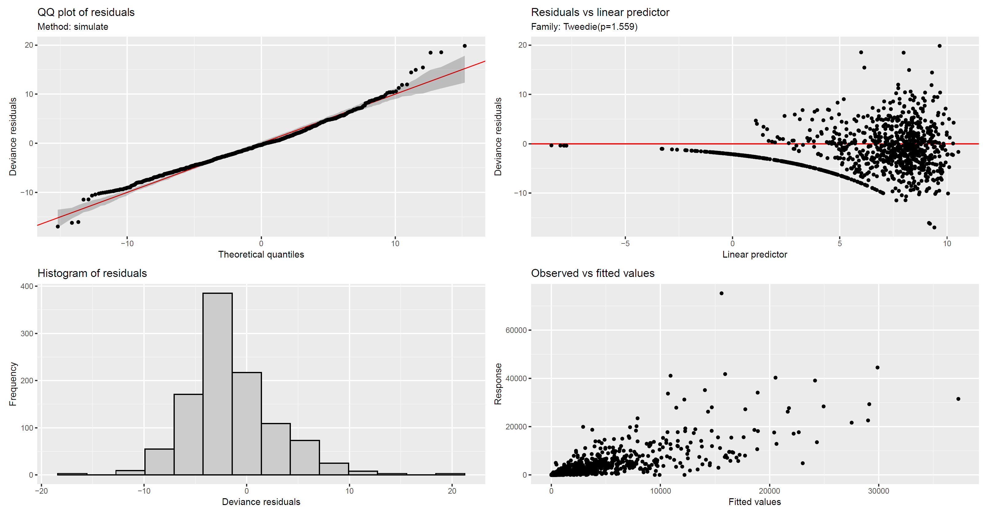
The plots Residuals vs linear predictor & Observed vs fitted values seem problematic, see linked plots image file:

Lastly, the concurvity check indicated that there are concurvity issues with s(LON, LAT) and s(abs(gebco)), as the values in the first (worst) line for these predictors almost equal 1:

                 para s(LON,LAT)    s(Year) s(abs(gebco))

worst    1.002761e-18  0.9976474 0.22243539     0.9976475
observed 1.002761e-18  0.2192788 0.03608689     0.9919063
estimate 1.002761e-18  0.1367153 0.20069831     0.9799472

Update:

Ηere's a new model with counts as a response variable and negative binomial as the family (the poisson does not look appropriate in the QQ plot):

gam_mod2 <- gam(TotalCatchNumber_round ~
                 s(LON, LAT, bs = "ds", k = 100) +
                 s(Year, bs = "gp", k = 10) +
                 s(abs(gebco), k = 10),
                offset = log(Surf), data = data, method = "REML", family = "nb")

and its summary:

Family: Negative Binomial(0.905) 
Link function: log 

Formula:
TotalCatchNumber_round ~ s(LON, LAT, bs = "ds", k = 100) + s(Year, 
    bs = "gp", k = 10) + s(abs(gebco), k = 10)

Parametric coefficients:
            Estimate Std. Error z value Pr(>|z|)    
(Intercept)  5.75400    0.09087   63.32   <2e-16 ***
---
Signif. codes:  0 ‘***’ 0.001 ‘**’ 0.01 ‘*’ 0.05 ‘.’ 0.1 ‘ ’ 1

Approximate significance of smooth terms:
                 edf Ref.df  Chi.sq p-value    
s(LON,LAT)    81.442 90.635 2184.25  <2e-16 ***
s(Year)        6.911  7.145  200.38  <2e-16 ***
s(abs(gebco))  5.073  6.074   62.25  <2e-16 ***
---
Signif. codes:  0 ‘***’ 0.001 ‘**’ 0.01 ‘*’ 0.05 ‘.’ 0.1 ‘ ’ 1

R-sq.(adj) =   0.39   Deviance explained = 78.5%
-REML = 5126.5  Scale est. = 1         n = 1061

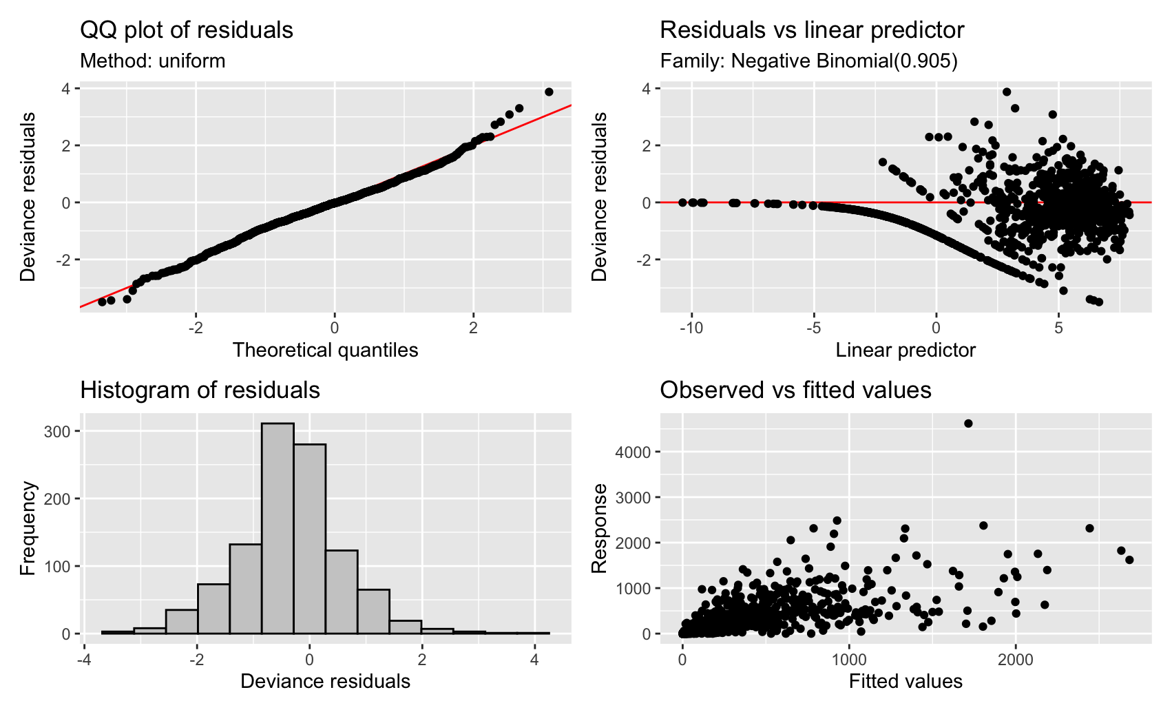
however, not much has changed, the diagnostics (gam.check results and plots and concurvity check) look largely the same:

Method: REML   Optimizer: outer newton
full convergence after 8 iterations.
Gradient range [-3.678611e-05,0.002145777]
(score 7291.597 & scale 1).
Hessian positive definite, eigenvalue range [1.461851,410.3035].
Model rank =  118 / 118 

Basis dimension (k) checking results. Low p-value (k-index<1) may
indicate that k is too low, especially if edf is close to k'.

                 k'   edf k-index p-value    
s(LON,LAT)    99.00 82.86    0.69  <2e-16 ***
s(Year)        9.00  6.93    0.77   0.005 ** 
s(abs(gebco))  9.00  4.88    0.78   0.005 ** 
---
Signif. codes:  0 ‘***’ 0.001 ‘**’ 0.01 ‘*’ 0.05 ‘.’ 0.1 ‘ ’ 1

                 para s(LON,LAT)    s(Year) s(abs(gebco))
worst    9.995557e-19  0.9976474 0.22243539     0.9976475
observed 9.995557e-19  0.1586361 0.05277781     0.9910242
estimate 9.995557e-19  0.1367153 0.20069831     0.9799472

I have also tried the Tweedie family with counts as a response variable, again no improvement.

Update #2

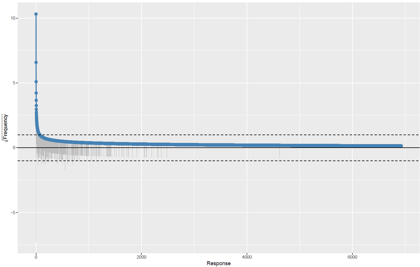
Here is the rootogram: According to from the bottom of the heap: rootograms, it does not look good, as all bars exceed the zero line (under prediction!).