Reference for Directional Statistics of Plane Orientation

Question

I've got a project I'm working on where I've got the orientation (normal) vectors of planes. These vectors are all within a unit hemisphere where the $z$-coordinate is strictly positive. The orientation can alos be given as the inclination angle $\theta_{inc}$ and the azimuth angle $\theta_{azi}$, written as $(\theta_{azi},\theta_{inc})$. Here, $\theta_{inc} \in [0,90^\circ]$ measured from the $z$-axis and $\theta_{azi} \in [0,360^\circ)$ measured from the $x$-axis. Any orientation of a plane in 3D space can be described by using these angles for normal vectors on this hemisphere. I would like to talk about how dispersed these vectors are, knowing that vectors near the $xy$-plane will wrap back around. In 2D the orientation of a line, with normal vector $v = \langle v_1,v_2\rangle$ where $v_1 \geq 0$, can be described uniquely by an angle $\theta = \arctan(v_2/v_1)$. The dispersion then of a collection of these angles can be quantified as the mean resultant length of the collection of the doubled angles. In other words, if $\Theta = \{\theta_1,\theta_2,...,\theta_n\}$ are a collection of slope angles, then the mean resultant length is the $$\overline{\Theta} = \frac{1}{n}\sqrt{\left(\sum_{i=1}^n \cos(2\theta_i) \right)^2 + \left(\sum_{i=1}^n \sin(2\theta_i) \right)^2}$$ However, I can't just double my inclination angle because different orientations would end up being assigned the same vector. For example, consider the orientations $(0,90^\circ)$, $(120^\circ,90^\circ)$, and $(240^\circ,90^\circ)$, which are all reasonably dispersed. If I double the inclination angle then all these orientations would be at an inclination of $180^\circ$. Here, the azimuth angle is degenerate, and the mean resultant length would be 1, indicating no dispersion. This is an obvious issue and requires either a very clever way of describing the periodicity of plane orientations OR perhaps an alternative way to compute the dispersion. I've tried to rummage around in the literature and I've been at a loss to find any references discussing this sort of thing, so recommendations for articles or books are much appreciated (neither the Ley-Verdebout text nor the Mardia-Jupp text seemed to help).

Answer 1

On spheres (embedded in Euclidean space), a natural and useful metric for comparing two points is based on the cosine of their included angle,

$$\delta(z_1,z_2) = 1 - z_1\cdot z_2$$

where $|z_1| = |z_2| = 1.$

The characterization of covariance at https://stats.stackexchange.com/a/18200/919 (in terms of a comparison of all distinct pairs of points in a dataset of size $n$) easily generalizes, because $z_i.z_i = |z_i|^2 = 1$ for all $i$ implies the mean distance is

$$\frac{2}{n(n-1)}\sum_{1\le i\lt j \le n} z_i \cdot z_j = \frac{1}{n(n-1)} \left[\left(\sum_{i=1}^n z_i\ \cdot\ \sum_{j=1}^n z_j\right) - n\right].$$

In your case, you require $\delta(z_i,z_j) = \delta(\pm z_i,\pm z_j)$ so you can ignore the directionality. The way to do that is to apply the absolute value to the left hand side. That is,

Summarize the dispersion of (unit-length) data as $$\sigma^2 = 1 - \frac{2}{n(n-1)}\sum_{1\le i\lt j \le n} |z_i \cdot z_j|.$$

This is justified as a measure of dispersion by virtue of its parallel with the (usual) covariance; and it is justified in its use for directional data because the rotation invariance of the dot product assures this summary is rotationally invariant.

Although the formula is inefficient (it cannot be simplified like the right hand side of the original equation), it's fast enough for many datasets because the sum can be expressed as a matrix product: putting the $z_i$ in rows of an $n\times p$ matrix $Z$ (where $p$ is the dimension of the coordinates, $p=3$ in your case), the expression for $\sigma^2$ is the mean of the upper triangular part of $ZZ^\prime.$ To be concrete, here is an R implementation. Its input is the array Z and its output in s2 is the value of $\sigma^2.$

  D <- tcrossprod(Z,Z)
  s2 <- 1 - mean(abs(D[upper.tri(D)]))

A practical limit for the dataset size is approximately 10,000 to 100,000 (because $ZZ^\prime$ then has $10^8$ to $10^{10}$ entries).

---

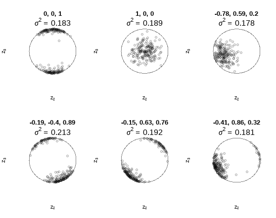
To illustrate, I generated six $\pm(z_1,z_2,z_3)$ datasets from a von Mises - Fisher distribution with concentration parameter $\kappa = 10$ and varying location parameters $\mu$ (given in the first lines of the headings). The signs were chosen to make $z_1$ nonnegative. These are plots of the projections of the data onto the $(z_2,z_3)$ plane.

Despite appearances to the contrary -- because these plots do not reflect the intrinsic nearness of (say) points near $(0,\cos\theta,\sin\theta)$ and diametrically opposite points close to $(0,-\cos\theta,-\sin\theta)$ -- all six datasets have nearly the same estimate of $\sigma^2.$ This shows how $\sigma^2$ correctly gives a consistent account of dispersion appropriate for your problem.