How to determine lambda for graphical lasso?

Question

I am trying to figure out how to determine lambda for a graphical lasso.

I have found that someone had the exact same question that me 9 years ago. I was wondering if anything exists in R to determine lambda in context of graphical lasso?

How to perform Cross-Validation for glasso to select lambda in R

Answer 1

The graphical LASSO (glasso) uses an $\ell_1$-norm penalized log-likelihood to obtain an estimate of $$\mathbf{\Theta} = \mathbf{\Sigma}^{-1},$$

the inverse variance-covariance matrix, or precision matrix.

The log-likelihood, as described in the original paper by Friedman, Hastie & Tibshirani (2008),$^1$ is equal to

$$\log \left( \det \left( \mathbf{\Theta} \right) \right) - \mathrm{trace}(\mathbf{S \Theta}) - \lambda ||\mathbf{\Theta}||_1$$

where $\mathbf{S}$ is an empirical estimate of $\mathbf{\Sigma}$ and $||\cdot||_1$ is the $\ell_1$-norm.

Several ways to determine the optimal value of $\lambda$ have been described in literature:

• Cross-validation;
• Extended Bayesian Information Criterion (EBIC);$^2$
• Stability Approach to Regularization Selection (StARS).$^3$

In addition, while not really providing an optimal value, the matrix condition number is a simple and effective tool to determine a lower bound for $\lambda$ by assessing the invertibility of $\mathbf{S}$. I also describe these methods to varying extends in my master's thesis, which is available online.$^4$

Choosing $\lambda$ through $k$-fold cross-validation

The easiest to implement (and perhaps also the easiest choice to defend) is by using a cross-validation loop. The idea is to estimate $\mathbf{\Theta}$ on the train set, and evaluate using an empirical estimate $\mathbf{S}$ of the test set. Other than that, it's mostly just trying to reproduce the log-likelihood formula above in R code.

Here is a quick implementation:

require("glasso")

kcv_glasso <- function(X, lambda, k = 10){
  fold <- sample(1:k, nrow(X), replace = TRUE)
  ll <- numeric(k)
  for(i in 1:k){
    train <- which(fold != i)
    test  <- which(fold == i)
    X_train     <- scale(X[train, ], center = TRUE, scale = FALSE)
    S_train     <- t(X_train) %*% X_train / length(train)
    Theta_train <- glasso(S_train, lambda)$wi
    logdetTheta <- determinant(Theta_train, logarithm = TRUE)[[1]][1]
    X_test <- scale(X[test, , drop = FALSE], 
                    center = attr(X_train, "scaled:center"), scale = FALSE)
    S_test <- t(X_test) %*% X_test / length(test)
    traceSTheta <- sum(diag(S_test %*% Theta_train))
    # The (penalized) log-likelihood:
    ll[i] <- logdetTheta - traceSTheta - lambda * norm(Theta_train, type = "1")
  }
  return(ll)
}

Let's try it out on two examples, one where we should not need any shrinkage ($n \gg p$) and one where we do ($n < p$).

Example: Invertible without shrinkage ($n \gg p$)

set.seed(2024)
X <- as.matrix(iris[, -5])
k <- 10
lambdas <- exp(seq(-20, 1, l = 100))
ll <- matrix(ncol = k, nrow = length(lambdas))
for(i in 1:length(lambdas)){
  ll[i, ] <- kcv_glasso(X = X, lambda = lambdas[i], k = k)
}
plot(rowMeans(ll, na.rm = TRUE) ~ lambdas,
     type = "l", bty = "n", log = "x", axes = FALSE,
     xlab = bquote(lambda), ylab = "log-likelihood", lwd = 3)
points(lambdas[which.max(rowMeans(ll, na.rm = TRUE))], 
       max(rowMeans(ll, na.rm = TRUE)), pch = 16, col = 2, cex = 1.5)
require("sfsmisc")
eaxis(1)
eaxis(2)

Example: Ill-defined without shrinkage ($n < p$)

set.seed(2024)
n <- 50
p <- 100
X <- matrix(rnorm(n * p), nrow = n, ncol = p)
k <- 10
lambdas <- exp(seq(-4, 4, l = 100))
ll <- matrix(ncol = k, nrow = length(lambdas))
for(i in 1:length(lambdas)){
  ll[i, ] <- kcv_glasso(X = X, lambda = lambdas[i], k = k)
}
plot(rowMeans(ll, na.rm = TRUE) ~ lambdas,
     type = "l", bty = "n", log = "x", axes = FALSE,
     xlab = bquote(lambda), ylab = "log-likelihood", lwd = 3)
points(lambdas[which.max(rowMeans(ll, na.rm = TRUE))], 
       max(rowMeans(ll, na.rm = TRUE)), pch = 16, col = 2, cex = 1.5)
eaxis(1, n.axp = 1)
eaxis(2)

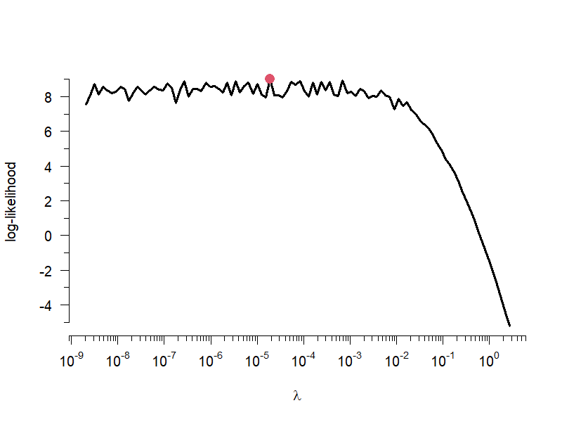
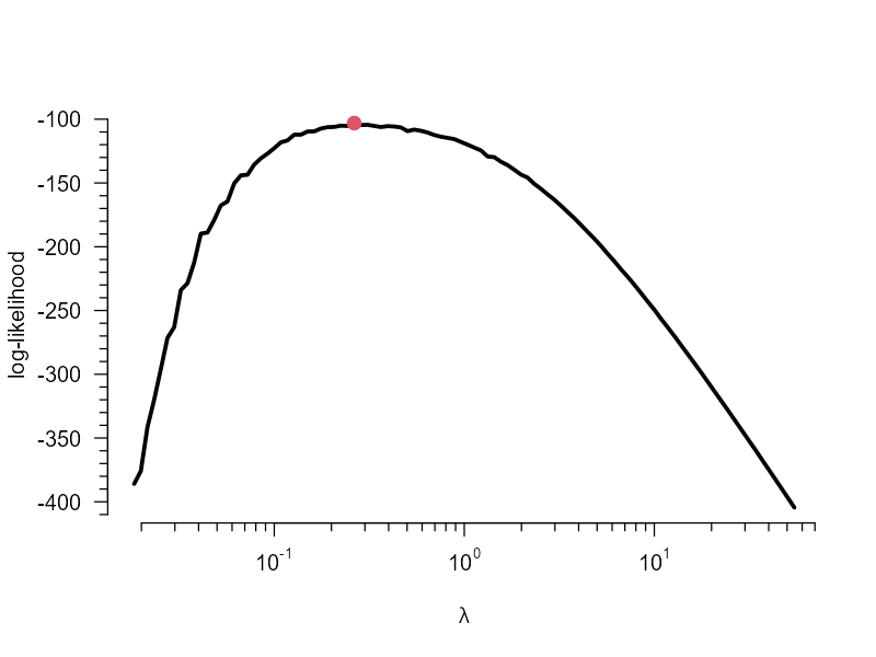
In the second example, we get a clear optimum of $\lambda$, whereas in the first example, any value, no matter how low, still results in a similar log-likelihood. You can also see there is considerable variability from splitting the data, so for a precise estimate of $\lambda$ it would be better to use multiple runs of $k$-fold cross-validation.

Some notes:

• Since you mentioned the study is exploratory in nature, and there is no apparent strong preference for glasso, consider the proper ridge penalized inverse covariance estimation implemented in the rags2ridges package. It uses a local false discovery rate (by default) to decide on the number of edges and has a built-in function for cross-validation. It also has the usual advantages over LASSO, including the ability to separate the estimation and variable-selection process, and less sensitivity to colinearity.
• If you have a small sample size, and want to use LOOCV, it is important to use the maximum likelihood estimate of $\mathbf{S}$ and not apply Bessel's correction.

---

1. Jerome Friedman, Trevor Hastie, Robert Tibshirani, Sparse inverse covariance estimation with the graphical lasso, Biostatistics, Volume 9, Issue 3, July 2008, Pages 432–441, https://doi.org/10.1093/biostatistics/kxm045
2. Foygel, R. & Drton, M. (2010). Extended Bayesian information criteria for Gaussian graphical models. Curran Associates Inc.
3. Liu, H., Roeder, K., & Wasserman, L. (2010). Stability Approach to Regularization Selection (StARS) for High Dimensional Graphical Models. Advances in neural information processing systems, 24(2), 1432–1440.
4. Rodenburg, F.J. (2017). A comparison of methods for the construction of conditional independence networks Leiden University Mathematical Institute (Thesis repository)