How to interpret coefficients of logistic regression using natural cubic splines?

Question

I'm trying to experiment with using natural cubic splines for logistic regression in R, and I'm having trouble interpreting and making use of the results.

For a variety of reasons, I need to be able to plot (and possibly further analyze) the results in Python. The problem is that while I can do this with standard logistic regression, I don't know how to do this for the case of logistic regression using (natural cubic) splines.

An example: doing logistic regression on the frequency of stellar bars in spiral galaxies, as a function of the total stellar mass of individual galaxies. (Here's a link to the data file, if you want to try fitting things yourself.)

If I do standard logistic regression with a quadratic logit function -- as I did with an earlier version of the dataset in Erwin 2018 [Github link to Python and R notebooks: https://github.com/perwin/s4g_barfractions], I get something like this in R (stripping away some of the output):

ff <- "barpresence_vs_logmstar_for_R_sp_w30_updateddist.txt"
logmstarBarSpTable <- read.table(ff, header=TRUE)

logMstarFitSp_quad <- glm(bar ~ logmstar + I(logmstar^2), 
                          family = binomial, logmstarBarSpTable)
summary(logMstarFitSp_quad)

Coefficients:
              Estimate Std. Error z value Pr(>|z|)
(Intercept)   -19.2096    26.0781  -0.737    0.461
logmstar        4.2945     5.3723   0.799    0.424
I(logmstar^2)  -0.2332     0.2760  -0.845    0.398
AIC: 828.4

I can easily plot the result in Python, since I know the "Coefficients" values correspond to coefficients in a quadratic equation: logit = beta_0 + beta_1*x + beta_2*x^2 where beta_0 = "(Intercept)", beta_1 = "logmstar", and beta_2 = "I(logmstar^2)", so the actual expression becomes logit = -19.2096 + 4.2945*x - 0.2332*(x**2) and then I can generate probability values with Python code like this: probability = 1.0 / (1.0 + np.exp(-logit))

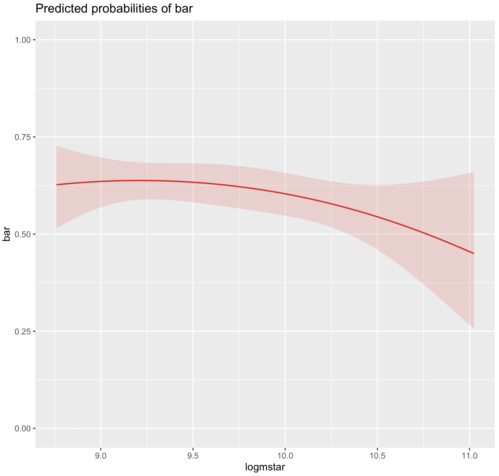
Here's the result of asking R to plot the fit, via plot_model(logMstarFitSp_quad, type = "pred", terms = c("logmstar"))

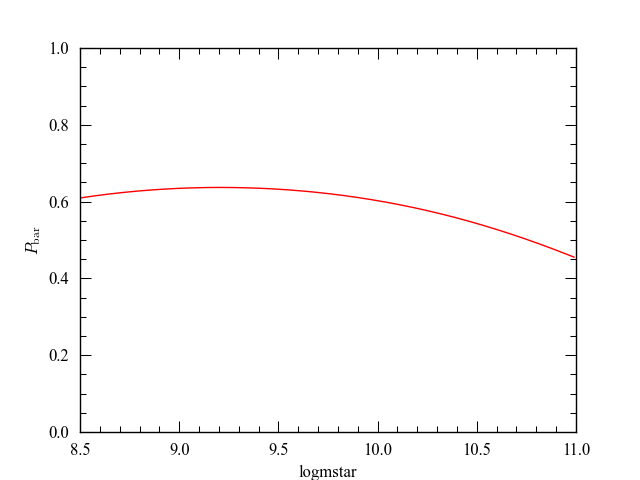
and here's the result of doing the same in Python, which agrees nicely:

def logit_quad( x, params=[-19.2096, 4.2945, -0.2332] ):
    return params[0] + params[1]*x + params[2]*(x**2)
xx = np.arange(8.5,11,0.01)
plt.plot(xx, 1.0 / (1.0 + np.exp(-logit_quad(xx)))

If on the other hand I try doing a simple natural-cubic-spline logistic regression in R (for simplicity, starting off with just one internal knot, so df=2) I get:

require("splines")
logMstarFitSp_spline2df <- glm(bar ~ ns(logmstar, 2),
                               family = binomial, logmstarBarSpTable)
summary(logMstarFitSp_spline2df)

Coefficients:
                 Estimate Std. Error z value Pr(>|z|)  
(Intercept)        0.5049     0.2285   2.210   0.0271 *
ns(logmstar, 2)1  -0.2487     0.5061  -0.492   0.6231  
ns(logmstar, 2)2  -0.7645     0.4276  -1.788   0.0738 .
AIC: 828.16

For what it's worth, I can figure out that the single internal knot is located at logmstar = 9.5575, via

str(attributes(summ$terms)$predvars)
 language list(bar, ns(logmstar, knots = c(`50%` = 9.5575), Boundary.knots = c(8.759, 11.024), intercept = FALSE))

... and I have no idea how to interpret this, or what the logit expression would look like in Python. What are the "Coefficients" in this model?

In principle, I think they should be the coefficients that multiply the basis functions of the spline, so that

   logit = beta_0*h_1(x) + beta_1*h_2(x) + beta_1*h_3(x)

where h_1, h_2, and h_3 are the three basis functions (and beta_0 = "(Intercept)", etc.).

But what are the basis functions? (My attempts to read the documentation for the R function ns have left me baffled; and I have not found much help in various spline-requested questions on this site.)

Answer 1

If you're willing to use rms::Glm instead of stats::glm, there is a much easier way to obtain the equations, by using Function, as described here.

If you do, there is another useful post here that explains the difference between restricted cubic splines fit with rms::rcs and splines::ns, and a post here with general guidance on understanding spline basis functions..

---

Conversely, if you don't care much for the mathematical expression and just want to be able to plot, just create a sequence of new $x$-values that span the range of the data, and then use predict:

x_seq  <- seq(8.5, 11, l = 1000)
y_pred <- predict(logMstarFitSp_spline2df,
                  newdata = data.frame(logmstar = x_seq), type = "response")

With a bit more work, you can also obtain the confidence band, by using predict(..., se.fit = TRUE), then using a normal approximation on the linear scale, then converting back to the original scale:

x_seq <- seq(8.5, 11, l = 1000)
pred <- predict(GLMlogMstarFitSp_spline2dfnewdata = data.frame(logmstar = x_seq), se.fit = TRUE)

# Compute a 95% CI, using a normal approximation on the linear scale
lwr  <- pred$fit + qnorm(0.025) * pred$se.fit
upr  <- pred$fit + qnorm(0.975) * pred$se.fit

# Convert back to the original scale
il <- binomial()$linkinv
newy <- cbind(il(pred$fit), il(lwr), il(upr))
plot(bar ~ logmstar, data = logmstarBarSpTable, pch = 16, bty = "n",
     xlab = "logmstar", ylab = bquote(P["bar"]))
lines(newy[, 1] ~ newx, lwd = 3, col = "red")
lines(newy[, 2] ~ newx, lwd = 1, col = "red", lty = "dashed")
lines(newy[, 3] ~ newx, lwd = 1, col = "red", lty = "dashed")