Moderate test statistic but low p-value in an F-test

Question

I am running a multiple regression on simulated data in R. The sample size is 100. There is one relevant regressor and 18 irrelevant ones. I am testing the joint significance of the 18 irrelevant regressors using Newey-West covariance matrix.

Puzzle 1: I find the 18 irrelevant regressors to be highly statistically significant.
Puzzle 2: I get a test statistic of 6.8814 under 18 degrees of freedom which seems moderate to me (not far out in the right tail of the F(18, 80) distribution), so how come this yields a very low p-value of 4.5e-10?

I was able to figure out puzzle 1. Apparently, Newey-West is the problem. Using vanilla covariance matrix, the result is much more sensible. However, I am still at a loss w.r.t. puzzle 2, and that is my question.

library(car)
library(sandwich)

m <- 20
n <- 100
set.seed(9999)
x <- rnorm(m * n)
X <- matrix(x, ncol = m)
X[, 2] <- X[, 1] + X[, 2]
# Now the 2nd column is the 1st column + some noise,
# while all the other columns are pure noise.
# Thus, if we try to predict the 1st column, then only the 2nd column should be helpful.
m1 <- lm(X[, 1] ~ X[, -1])
(test <- linearHypothesis(
  model = m1,
  hypothesis.matrix = (diag(m)[-c(1:2), ]),
  rhs = rep(0, m - 2),
  test = "F",
  vcov. = NeweyWest(m1)
))

Result:

Linear hypothesis test

Hypothesis:


Model 1: restricted model
Model 2: X[, 1] ~ X[, -1]

Note: Coefficient covariance matrix supplied.

  Res.Df Df      F    Pr(>F)    
1     98                        
2     80 18 6.8814 4.494e-10 ***

Without the Newey-West:

(test <- linearHypothesis(
  model = m1,
  hypothesis.matrix = (diag(m)[-c(1:2), ]),
  rhs = rep(0, m - 2),
  test = "F"
))

Result:

Linear hypothesis test

Hypothesis:


Model 1: restricted model
Model 2: X[, 1] ~ X[, -1]

  Res.Df    RSS Df Sum of Sq      F Pr(>F)
1     98 38.856                           
2     80 31.982 18    6.8739 0.9552 0.5178

Edit 1: Thank you to Lukas Lohse for a good comment. When evaluating the size of the test statistic informally, I was thinking of the $\chi^2$ approximation to the $F$ distribution but forgot that I have to multiply the $F$ value by the numerator degrees of freedom (here, 18) to get the corresponding $\chi^2$ statistic... OK, so instead of puzzle 2 we now have a new puzzle 3: why does the test with Newey-West use 6.8 as the $F$-statistic and the one with vanilla variance estimator as the sum of squares.

Edit 2: It looks like puzzle 3 was based on a coincidence where the $F$-statistic and the sum of squares just happened to be close. Lukas Lohse has the answer.

Answer 1

Ok, so I've looked at it quite a bit. I don't have a final answer but I think I'm calling it here.

I removed the real association from the data generation and added 2 additional robust variance estimators, HC3 and default HAC. What I found is that the F-statistic and the sum of squares being identical appears to have been a large coincidence but the robust variance estimators actually shrink the standard errors (I used lmtest::coeftest) by some degree and by extension inflate the F-statistic.

library(car)
library(sandwich)

m <- 20
n <- 100
set.seed(9999)
x <- rnorm(m * n)
X <- matrix(x, ncol = m)
y <- rnorm(n) 
m1 <- lm(y ~ X)

linearHypothesis(
  model = m1,
  hypothesis.matrix = (diag(m+1)[-1,]),
  rhs = rep(0, m),
  test = "F"
) # F = 1.4 (Sum of Sq = 29.3)

linearHypothesis(
  model = m1,
  hypothesis.matrix = (diag(m+1)[-1,]),
  rhs = rep(0, m),
  test = "F",
  vcov. = hccm(m1, type = "hc3")
)# F = 1.8

linearHypothesis(
  model = m1,
  hypothesis.matrix = (diag(m+1)[-1,]),
  rhs = rep(0, m),
  test = "F",
  vcov. = vcovHAC(m1)
)# F = 2.5

linearHypothesis(
  model = m1,
  hypothesis.matrix = (diag(m+1)[-1,]),
  rhs = rep(0, m),
  test = "F",
  vcov. = NeweyWest(m1),
  verbose = F
)# F = 5.5


library(lmtest)
coeftest(m1)
coeftest(m1, vcov.=NeweyWest(m1))
se_lm <- coeftest(m1)[, 2]
se_hc <- coeftest(m1, vcov.=vcovHAC(m1))[, 2]
se_nw <- coeftest(m1, vcov.=NeweyWest(m1))[, 2]
plot(se_lm, se_nw, ylim = c(0.05, 0.2))
points(se_lm, se_hc, col = 2)
abline(0,1)

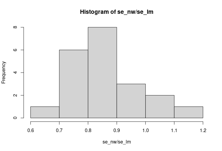
hist(se_nw/se_lm)

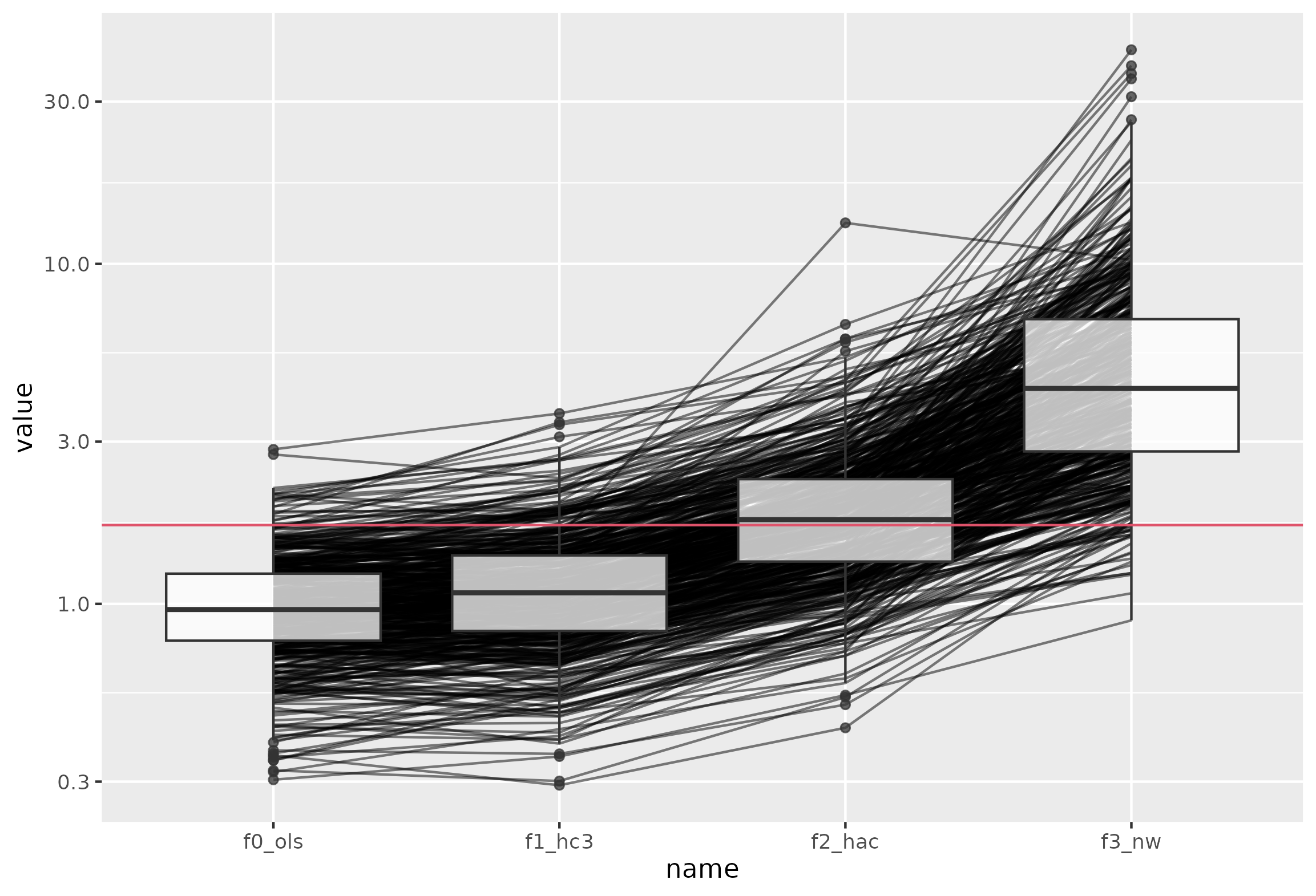
I also ran 500 simulations and produced this plot of the F-statistics with the 4 methods. We can clearly see that Newey West is by far the worst offender, but they all inflate. The picture is much more extreme if we set m = 30.

What's going on?

The only thing I could find is this: https://stats.stackexchange.com/a/590851/341520

Apparently for small samples (our example has about 5 observations per coefficient) robust standard errors can substantially underestimate. Sadly I don't really understand the paper linked in the other answer.

Code for 2nd image

m <- 20
n <- 100
# ~ 1 minute run time
dat <- t(replicate(500, {
  x <- rnorm(m * n)
  X <- matrix(x, ncol = m)
  y <- rnorm(n) 
  m1 <- lm(y ~ X)
  f0_ols <- linearHypothesis(
    model = m1,
    hypothesis.matrix = (diag(m+1)[-1,]),
    rhs = rep(0, m),
    test = "F"
  )$F[2]
  
  f1_hc3 <- linearHypothesis(
    model = m1,
    hypothesis.matrix = (diag(m+1)[-1,]),
    rhs = rep(0, m),
    test = "F",
    vcov. = hccm(m1, type = "hc3")
  )$F[2]
  
  f2_hac <- linearHypothesis(
    model = m1,
    hypothesis.matrix = (diag(m+1)[-1,]),
    rhs = rep(0, m),
    test = "F",
    vcov. = vcovHAC(m1)
  )$F[2]
  
  f3_nw <- linearHypothesis(
    model = m1,
    hypothesis.matrix = (diag(m+1)[-1,]),
    rhs = rep(0, m),
    test = "F",
    vcov. = NeweyWest(m1),
    verbose = F
  )$F[2]
  c(f0_ols = f0_ols, f1_hc3 = f1_hc3, f2_hac = f2_hac, f3_nw = f3_nw)
}))

#dat 
library(tidyverse)
dat %>% 
  data.frame() %>% 
  rowid_to_column() %>% 
  pivot_longer(cols = -1) %>% 
  ggplot(aes(x = name, y = value)) +
  geom_path(aes(group = rowid), alpha = 0.5) +
  geom_boxplot(alpha = 0.75) +
  geom_hline(yintercept = qf(0.95, 20, 79), col = 2) +
  scale_y_log10()