How to decide to include interactions just by looking at the data?

Question

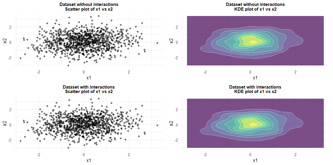
I am having a bit of a hard time to understand how to interpret and understand interaction terms in regression models. I have made an R example to show where I am confused (https://www.dropbox.com/scl/fi/yxf1n75dfdta45q8pj3vz/dropbox_code-1-1.txt?rlkey=gazzbhach9i5q3m1nkf01g9l4&st=lptm3zgr&dl=0).

Suppose I have two datasets - one of them is created without interactions and the other is created with interactions:

n <- 1000
x1 <- rnorm(n)
x2 <- rnorm(n)
x3 <- rnorm(n)    
    
# Dataset 1: y is a function of x1, x2, x3 without interactions
y1 <- 2 + 0.5*x1 + 0.3*x2 + 0.7*x3 + rnorm(n, 0, 0.5)
# Dataset 2: y is a function of x1, x2, x3 with interactions
y2 <- 2 + 0.5*x1 + 0.3*x2 + 0.7*x3 + 0.4*x1*x2 + 0.2*x1*x3 + 
       0.1*x2*x3 + rnorm(n, 0, 0.5)
    
df1 <- data.frame(y = y1, x1 = x1, x2 = x2, x3 = x3)
df2 <- data.frame(y = y2, x1 = x1, x2 = x2, x3 = x3)

These interactions are not immediately clear to me when looking at the scatter plots:

Then, I fit 4 regression models to cover all combinations:

# Fit regression models for Dataset 1
model1_without_int <- lm(y ~ x1 + x2 + x3, data = df1)
model1_with_int <- lm(y ~ x1 * x2 * x3, data = df1)    
    
# Fit regression models for Dataset 2
model2_without_int <- lm(y ~ x1 + x2 + x3, data = df2)
model2_with_int <- lm(y ~ x1 * x2 * x3, data = df2)

Doing this, it looks like the interaction terms are significant in the model that was fit on the data with interactions:

Dataset 1 Interaction Estimates:
> print(summary(model1_with_int)$coefficients[c("x1:x2", "x1:x3", 
    "x2:x3"), ])
          Estimate Std. Error    t value   Pr(>|t|)
x1:x2  0.002490521 0.01574894  0.1581389 0.87437950
x1:x3 -0.027456680 0.01637998 -1.6762337 0.09400753
x2:x3 -0.034349287 0.01675775 -2.0497550 0.04065083
> cat("\nDataset 2 Interaction Estimates:\n")

Dataset 2 Interaction Estimates:
> print(summary(model2_with_int)$coefficients[c("x1:x2", "x1:x3", 
    "x2:x3"), ])
        Estimate Std. Error   t value      Pr(>|t|)
x1:x2 0.39563591 0.01585618 24.951520 4.811481e-107
x1:x3 0.18470379 0.01649152 11.199922  1.682661e-27
x2:x3 0.06967006 0.01687187  4.129363  3.943817e-05

As I see it, the interaction coefficient of 0.39 means that for each one-unit increase in x1, the effect of x2 on y increases by 0.39 units, and vice versa. Suppose the main effects are (x1): 0.5 and (x2): 0.3. With the interaction term, the effects would be:

• Effect of x1 = 0.5 + 0.39 * x2
• Effect of x2 = 0.3 + 0.39 * x1

Also, it seems that the model with interactions fits better on the dataset with interactions and the model without interactions fits better on the data without interactions:

                              Model      AIC      BIC Residual_Sum_of_Squares
    1   Dataset 1 - No Interactions 1442.595 1467.134                245.2979
    2 Dataset 1 - With Interactions 1442.326 1486.496                243.2780
    3   Dataset 2 - No Interactions 2044.821 2069.359                447.9577
    4 Dataset 2 - With Interactions 1455.899 1500.069                246.6025

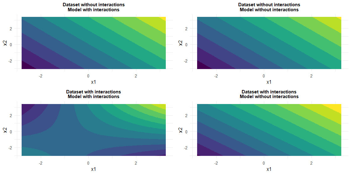
I then looked at the contour plots of the interactions for all 4 models:

The curved contours are a sign of interactions apparently (I am not fully sure why)

My question is : Why are the interactions so visible the contour plots but not in the raw data? By looking at the data without fitting the model, how can I decide to include interactions? Is this only possible post-hoc?

Answer 1

I think a strong case can be made for deciding on whether to include interactions before even looking at the data. You should certainly decide whether to examine them before looking at data, unless you are doing purely exploratory work (or are splitting your data into train, test, and possibly verify.

Your last table with the AIC values is to be expected. Note that the model with interactions has almost the same AIC as the one without, on the datset without interactions. This follows from the formula for AIC.

As to the plots, well:

1. If you wanted to just use the data, you could make trellis plots. They would have to include all three variables (or more, if you have more). There are other methods, too, such as using color to code the other variable. But the plots you show at the top can't show the interaction. The interaction is a different relation between x1 and y at different levels of x3 (also, different relation between x2 and y at different levels of x1). Your plots don't even look at that.

2. Contour plots are designed, in part, to look for interactions. Note that the plots include all three variables.