p-values for hypothesis testing

Question

Intuitively, the p-value in a standard hypothesis test (where the test statistic is either normally, or approximately normally distributed) is thought of as the "probability of observing a value at least as extreme as the one the statsitician observes, given the null is true".

My issue comes from the "at least as extreme part". This is due to using the complement of the CDF of the value at the test statistic. This implies that we are considering other, more extreme (and irrelevant) values of a test statistic we do not observe. Why is not using the pdf of the test statistic enough ? I worry that in rejecting a null, we are considering the extreme values which are not relevant for the particular test.

Answer 1

The p-value is sometimes criticised (mostly by people who prefer Bayesian inference) for being dependent on the "more extreme" part and thus on values that were not observed. However, that is a nonsense criticism because most statistical methods that do not utilise p-values also depend on values that were not observed.

Most statistical methods utilise a statistical model when evaluating the meaning and nature of observed values. The statistical model will typically entail or specify a set of values that the observations might take, and selection of a statistical model for any inferential problem is (should be) influenced by whether that set of values is 'reasonable' in some sense. Thus a method based on such a model will always depend on values that were not observed.

It might be that the p-value is criticised for being dependent on values not observed because the usual definition – correct, but often not particularly helpful – specifies "or more extreme". An alternative way of defining the p-value, mathematically equivalent, can make that sound less intrusive: a p-value is the fractional ranking of the observed value of the test statistic among all values of test statistic predicted by the statistical model. A p-value of 0.012 results from the observed test statistic being at the upper 1.2 percentile. (This fractional ranking definition is most easily understood with one-tailed p-values. For two-tailed p-values it is necessary to specify that the sign of the difference between the observed test statistic and the null hypothesised value is ignored.)

Likelihood-based methods of inference derive more directly from the pdf or pmf of the test statistic and they are worthy of consideration in many cases. However, it is important to recognise that the pdf and pmf functions are those predicted by the model and so even likelihood methods are not entirely without some influence of unobserved values.

A simple and incomplete comparison of the p-value and likelihood methods might help you where you say that the more extreme values are "not relevant". The same model can be used for p-values and likelihoods. To get a p-value you have to 'nail down' the potential parameter space to the null hypothesised value, and then you consider the observed value of the test statistic relative to all other possible values. In a likelihood analysis the likelihoods of parameter values are considered after the test statistic value is 'nailed down' to the observed value and the likelihoods of interesting parameter values are compared with each other.

Answer 2

The interpretation of only the pdf or pmf values can be ambiguous. For example, they can have very small values and need to be compared in a certain relative sense.

Using the CDF is one way. Another is to use the likelihood ratio.

Is the exact value of any likelihood meaningless?

Why is everything based on likelihoods even though likelihoods are so small?

---

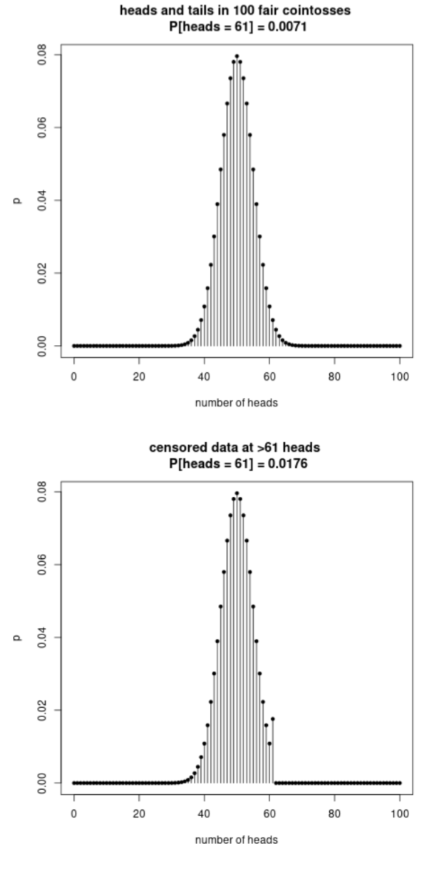
Example case study. Imagine you wish to test whether a coin is fair by tossing it 100 times and count the number of heads. If you observed 61 heads, then would it matter whether you had a censored measurement or uncensored measurement in which cases $P[heads=61]$ are not the same?

In this example the probabilities are different 0.0071 vs 0.0176, but the conclusions are arguably the same. The exact probabability/likelihood of the observation measurement is not the relevant value.

---

Interesting related topics are the differences between confidence intervals and credible intervals and the differences between likelihood/posterior and fidicial probability.

We can regard the distribution in multivariate way as a function of both parameter and estimate $F(\theta,\hat\theta)$. The differences between the methods depend on how we slice that function in single variate functions. See for example: What does "fiducial" mean (in the context of statistics)?.

This question and it's language...

other, more extreme (and irrelevant) values of a test statistic

values which are not relevant for the particular test.

... it relates a lot to the discussions about the likelihood principle.

The reason for using those 'irrelevant' values is because fiducial probability, p-values, and confidence intervals answer a different question, or at least use a different approach (they condition on the parameters instead of on the observation). See the question and answer here: An example where the likelihood principle really matters?

Answer 3

Michael Lew's answer mentioned partly about the criticism pertinent to the definition of $p$‐value, but didn't expound on that point (which is okay as the answer was addressing from a different pov with an alternate interpretation in tandem with the mathematical definition).

For the sake of argument, as OP raised a reasonable objection, it is deemed apt to address how the very dependence on extreme values which actually haven't been observed somewhat befuddles using $p$–value as "strength of evidence" against a (null) hypothesis.

It is known from the law of likelihood that the evidence associated with an observation $\mathbf X=\mathbf x$ concerning the hypothesis $\mathrm H_0:\theta=\theta_0$ vis-à-vis $\mathrm H_1:\theta=\theta_1$ is $f(\mathbf x;\theta_0) /f(\mathbf x;\theta_1); $ no other information -- whether thhose being the possible values of $\mathbf X$ that have not been realized or any other aspect -- should not be relevant for measuring the evidence for $\mathrm H_0$ vis-à-vis $\mathrm H_1.$

This leads to the principle of irrelevance of the sample space: consider an experiment involving tossing of a coin $20$ times to gather evidence about the possible value of $\theta, $ the probability of heads appearing in a toss. There are two investigators: $A$ and $B$. The result of the experiment is reported as the total number of heads obtained to $A$ while $B$ only gets to know whether the number of heads is $6$ or not.

When the experiment results in $6, $ the evidence concerning $\mathrm H_0:\theta=\theta_0$ vis-à-vis $\mathrm H_1:\theta=\theta_1$ is same for both $A$ and $B;$ that is the likelihood ratios for both the investigators are same: $\theta_0^6(1-\theta_0)^{14}/\theta_1^6(1-\theta_1)^{14}.$ Had the experiment reulted in a different number of heads other than $6, $ the evidence obtained would be different for each investigators. But that is irrelevant now that the realized observation is $6.$

As Royall in $[\rm I]$ writes (emphasis mine):

Although the scientific community might reasonably have chosen to subscribe to [$A$] in preference to [$B$], on the grounds that [$A$] could promise to provide a more detailed description of the observation under most circumstances, for the result that actually occurred, six heads, [$B$'s] report is equivalent, as evidence about $\theta,$ to [$A$'s]. Any concept or technique for evaluating observations as evidence that denies this equivalence, attaching a different measure of ‘significance’ to [$A$] of this result than to [$B$], is invalid. Whatever can be properly inferred about $\theta$ from [$A$] can be inferred from [$B$] and vice versa. The difference between [the two] sample spaces is irrelevant. ... The ‘irrelevance of the sample space’ is a critically important concept, for it implies a structural flaw that is not limited to significance tests, but pervades all of today’s dominant statistical methodology.

That is, a proper measure of evidence should not depend on the probabilities of unrealised "extreme" values. But $p$–value relies on the probabilities of those very extreme outcomes which didn't occur.

This does impact the prospect of using $p$–value as a measure of evidence.

Suppose in the above experiment $\rm H_0: \theta=0.5 $ and $\rm H_1:\theta<0.5.$ The test statistic is the total number of heads and small values would be considered extreme as they would be implausible under $\rm H_0.$ When $\rm x=6, $ both $A$ and $B$ would have the same information as the prior probability ratio $\Pr(\rm H_0) /\Pr(H_1) $ would be increased by $f(6;0.5) /f(6;\theta_1). $ However the $p$–value would be different:

• in case of $A:$ $$\Pr[6~\textrm{or less number of heads}\mid \theta=0.5]=0.06, $$

• in case of $B:$ $$\Pr[6\mid \theta=0.5]=0.04,$$ since for $B$ in $\{6, ~\text{not}~6\}, $ the extreme event is $6.$

This leads to an illogical conclusion:

The $p$–values assert (incorrectly) that the outcome (six heads in $20$ tosses) is stronger evidence against $\rm H_0$ (in favor of $\rm H_1$) for [$B$] than it is for [$A$].

Royall, in that vein, writes:

The significance-test approach to measuring the evidence is wrong because its dependence on the sample space leads to different answers in situations where the evidence is the same. That is, it violates the principle of the ‘irrelevance of the sample space’.

Perhaps more compelling is what Jeffreys stated:

... a hypothesis which may be true may be rejected because it has not predicted observable results which may have not occured.

--

References:

$\rm[I]$ Statistical Evidence : A Likelihood Paradigm, Richard M. Royall, Chapman& Hall, $1997,$ sec. $1.11, 3.4.$

$\rm[II]$ Introductory Statistical Inference with the Likelihood Function, Charles A. Rhode, Springer International, $2014, $ sec. $5.3.$

Answer 4

"Intuitively, the p-value in a standard hypothesis test (where the test statistic is either normally, or approximately normally distributed)"

First, the test statistic does not need to be normally or approximately distributed. It can have many kinds of distributions.

As far as the "at least as extreme" part, this is a parametric test and as such, unobserved values have to be considered. Also, the meaning of the p-value has to be consistent with the alternative hypothesis. In a Null Hypothesis Significance Test (NHST), the alternative hypothesis includes extreme values. Therefore, the p-value has to account for them. Moreover, if the model is continuous, using the pdf to get a probability for getting the exact observed value under the null hypothesis would be 0.

Answer 5

I'm going to focus on what seems to be your question. As you stated: "This implies that we are considering other, more extreme (and irrelevant) values of a test statistic we do not observe. Why is not using the pdf of the test statistic enough ?"

In the context of statistics that are normally distributed (or simply continuous), just looking at the probability of getting a statistic exactly as extreme as (i.e. equal to) what you got does not give you anything because that probability is exactly 0.

More generally, the idea of p-value testing is Step 1: You assume Ho, determine the distribution of your test statistic under this Ho and set the significance level $\alpha$. Step 2: Gather your evidence and compute your test statistic. Using the distribution under the null, compute the probability of getting at least as extreme as the statistic you got, i.e. the p-value. Step 3: If this p-value is small, it means that under your assumed null, it seems that it is very unlikely to get this value or more extreme values. Hence, you conclude that your initial assumption must be false (i.e. reject Ho)! This last step likewise shows why it is important to get the tail probability, not just the probability at the value, even if we were talking about discrete statistics.