For didactic reasons, I will use bootstrapping the sample mean as an example. All arguments are valid for other statistics (like a regression slope). I will also use the boot package instead of your (correct) manual implementation of the bootstrap.
First, let's remember, what the statistic of the Welch t-test is:
$t = \frac{\bar{x_1} - \bar{x_2}}{\sqrt{\left(\frac{s_1}{\sqrt{n_1}}\right)^2 + \left(\frac{s_2}{\sqrt{n_2}}\right)^2}}$
where $\frac{s_j}{\sqrt{n_j}}$ are the standard errors of the means. This formula of the standard error is valid for samples from a normal distribution, which is a basic assumption of the t-test.
Looking at the formula of $t$ we can see that if the sample means and standard deviations are kept constant and the sample sizes increase, $t$ increases and consequantly, the p-value decreases. (In fact, analysis of power is based on this.)
Now, what is the purpose of the bootstrap? We use the bootstrap to infer something about the distribution of a statistic derived from a sample, without having to make strong assumptions about the distribution from which the sample was taken (like it is necessary for the t-test). For example, we can use bootstrap to estimate the standard error of the sample mean. A basic property of the bootstrap method is that if we increase the size of the bootstrap resamples, this estimate approaches a fixed value asymptotically (Efron, 1979).
You can derive p-values from the bootstrap (https://stats.stackexchange.com/a/277391/11849). However, doing a t-test with the bootstrap resamples as in your example doesn't test $H_0: \mu_1 = \mu_2$, i.e., if the original samples are derived from distributions with equal means. It is nonsense, because the result depends on the size of the bootstrap resamples.
Having said all of this, let's look at an example:
set.seed(42) #for reproducibility

x1 <- rnorm(100)
x2 <- rnorm(100)

#t-test
print(t_test <- t.test(x1, x2))
#   Welch Two Sample t-test
#
# data:  x1 and x2
# t = 0.87011, df = 194.18, p-value = 0.3853
# alternative hypothesis: true difference in means is not equal to 0
# 95 percent confidence interval:
#  -0.1519980  0.3919951
# sample estimates:
#   mean of x   mean of y
#  0.03251482 -0.08748371
The Welch t-test gives a non-significant p-value as expected. The R function helpfully shows the sample means. Obviously, these will always be different for the two samples, even though the samples are from the same distribution. Nevertheless, the sample mean is an estimator of the distribution mean.
m1 <- mean(x1)
m2 <- mean(x2)
se1 <- sd(x1)/sqrt(100)
se2 <- sd(x2)/sqrt(100)
Now, let's bootstrap these means with increasing sizes of the bootstrap resamples:
library(boot)
nboot <- ((1:25) *10)^2
myboots <- lapply(nboot, function(n, x1, x2) {
  cbind(
    boot(x1, function(x, i) mean(x[i]), n)$t,
    boot(x2, function(x, i) mean(x[i]), n)$t
  )
}, x1 = x1, x2 = x2)
We can now plot the bootstrap means:
bootmeans <- sapply(myboots, function(x) colMeans(x))

matplot(nboot, t(bootmeans), pch = 16, main = "bootstrap means")
legend("center", pch = 16, col = 1:2, legend = c("sample 1", "sample 2"))
abline(h = m1, col = 1)
abline(h = m2, col = 2)
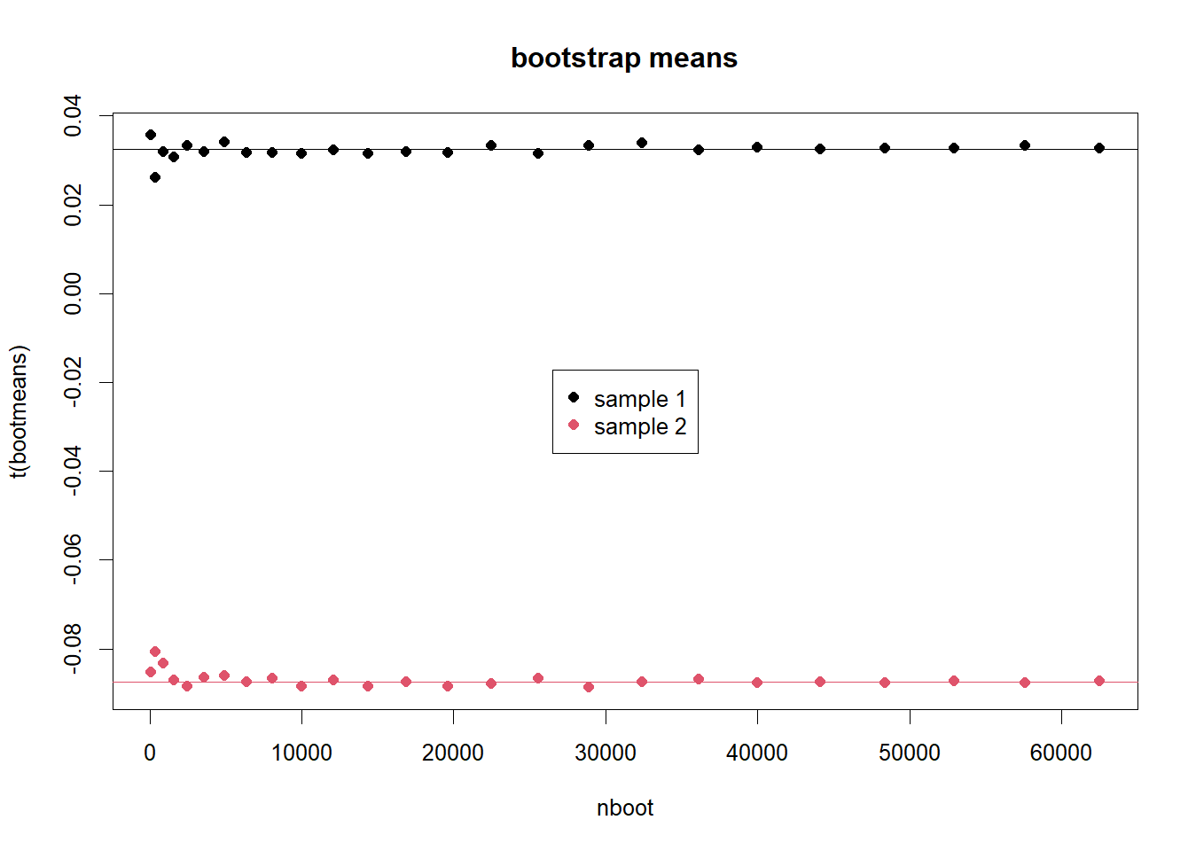
We can nicely see that with increasing bootstrap n the bootstrap means approach the sample means and bias is very low.
The same for the standard deviations, which are an estimate of the standard errors of the means:
bootSE <- sapply(myboots, function(x) apply(x, 2, sd))
matplot(nboot, t(bootSE), pch = 16, main = "bootstrap standard errors")
legend("top", pch = 16, col = 1:2, legend = c("sample 1", "sample 2"))
abline(h = se1, col = 1)
abline(h = se2, col = 2)
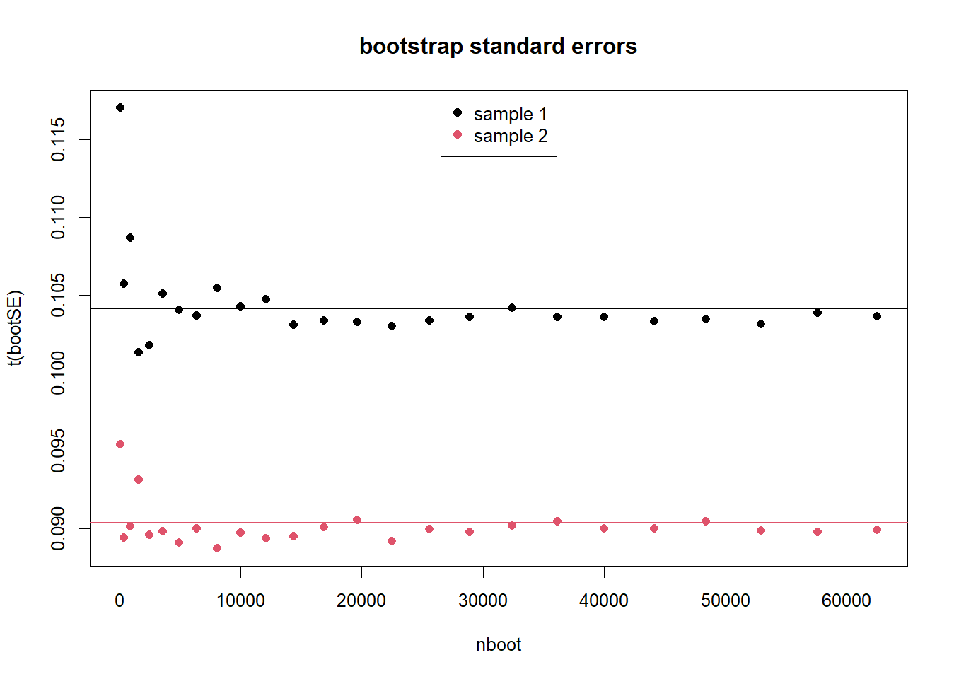
We see that they approach values close to the estimates based on the original samples and the assumption of normal distribution. We can also look at t-values:
plot(nboot, (bootmeans[1,] - bootmeans[2,])/sqrt(bootSE[1,]^2 + bootSE[2,]^2), pch = 16, main = "bootstrap t-values")
abline(h = t_test$statistic, col = 1)

Again, these are pretty constant for large bootstrap n and agree quite well with the t-test on the orginal samples.
Now, what went wrong in your approach?
Well, by using the t.test functions with the bootstrap resamples, you have an additional division by the square root of the bootstrap n. I will plot these wrong t-values against the square root of bootstrap n (different x-axis than the other plots).
plot(sqrt(nboot), (bootmeans[1,] - bootmeans[2,])/sqrt(bootSE[1,]^2/nboot + bootSE[2,]^2/nboot), pch = 16, main = "wrong t-values")
legend("bottom", pch = 16, col = 1:2, legend = c("sample 1", "sample 2"))

As you see these t-values will go to infinity if you increase the size of the bootstrap resamples. Consequently, p-values will approach zero.
Finally, your last plot shows strongly overlapping histograms. The plot doesn't show a significant difference.
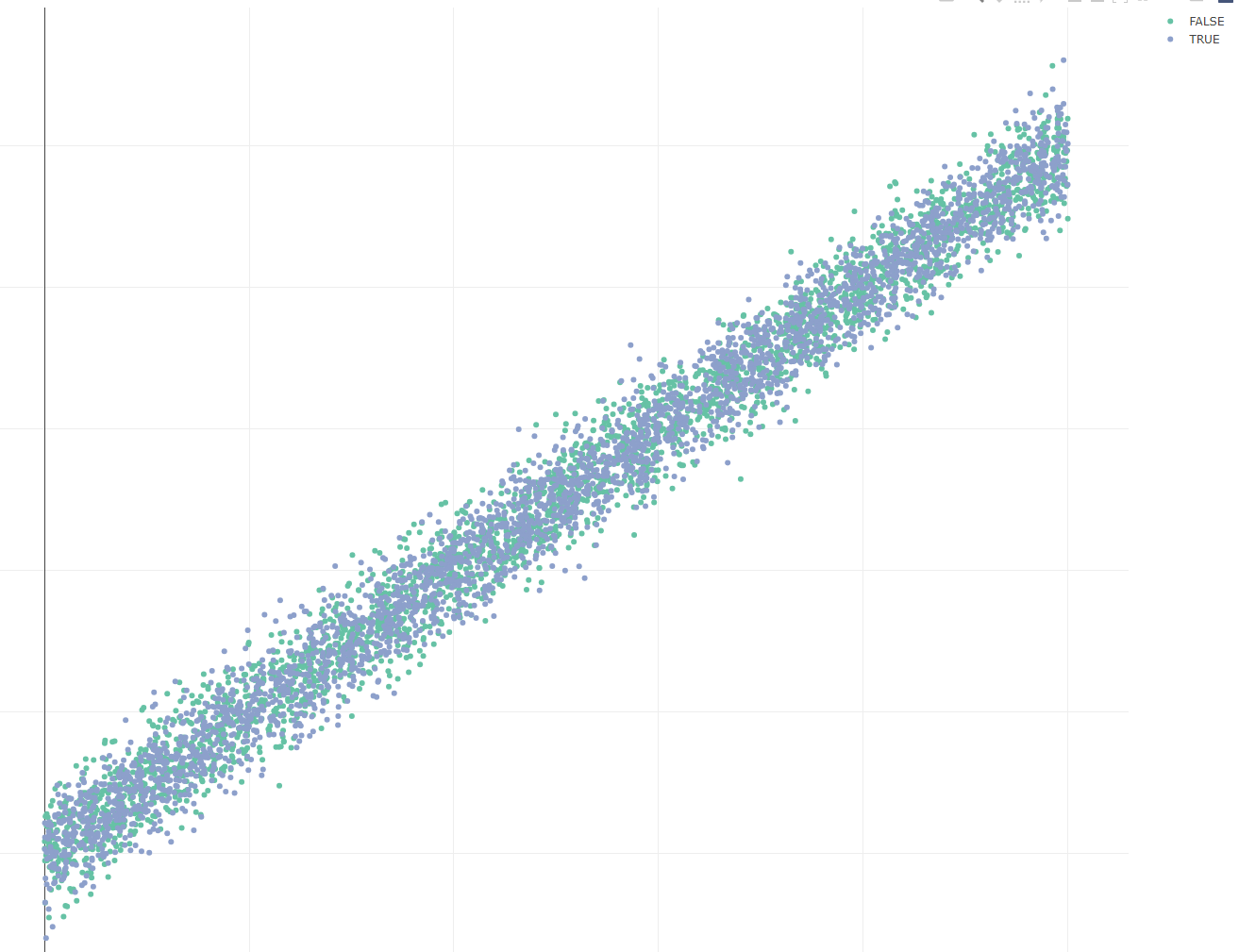 Here we do not have a difference as is comming from the same population (as shown by the first T-test) what is expected


yandy2. $\endgroup$N) and different boot strap numbers (different numbers forsize). I have been playing around with the code for a bit and I am too struggling to understand why that is the case. $\endgroup$