The plot of a single chi square RV approaches infinity at X^2 = 0. Why is that when chi square RVs are added, the resulting pdf plot seems to be at a finite value at Y= 0, where Y = the sum of these RVs. Also, various sources say that a chi square RV with 2 dgf is actually an exponentially distributed RV. Chi square RVs are generally associated with distribution of variances whereas exponentially distributed RV is often associated with the probability of time until next event. So, how do we resolve these two seemingly different interpretations so that they qualitatively describe the same thing? I'm not looking for a full technical mathematical proof but instead a general qualitative intuition.
-
$\begingroup$ It is not a complete answer but the images about the ambiguity of densities, from this answer, might help a bit. Squaring a variable can change the density from zero to infinity, in the point $X=0$. $\endgroup$– Sextus EmpiricusCommented Nov 17 at 1:12
-
1$\begingroup$ A $\chi^2_k$ distribution (so with $k$ degrees of freedom, the sum of $k$ iid $N(0,1)$ random variables) has the same density as a gamma distribution with shape parameter $\frac k2$ and scale parameter $2$, so as $x \to 0^+$ its density tends: towards $\infty$ when $\frac k2 < 1$ i.e. $k<2$; towards a finite positive value when $\frac k2 = 1$ i.e. $k=2$; and towards $0$ when $\frac k2 > 1$ i.e. $k>2$. $\endgroup$– HenryCommented Nov 17 at 1:38
-
2$\begingroup$ For a purely mathematical account of how singular functions can become tractable in higher dimensions (which is what is happening with the convolution of the densities), see my post at math.stackexchange.com/a/15462/1489. This is a general explanation of what @Sextus has so nicely illustrated in this thread for a special case. $\endgroup$– whuber ♦Commented Nov 17 at 15:25
1 Answer
The plot of a single chi square RV approaches infinity at X^2 = 0. Why is that when chi square RVs are added, the resulting pdf plot seems to be at a finite value at Y= 0, where Y = the sum of these RVs.
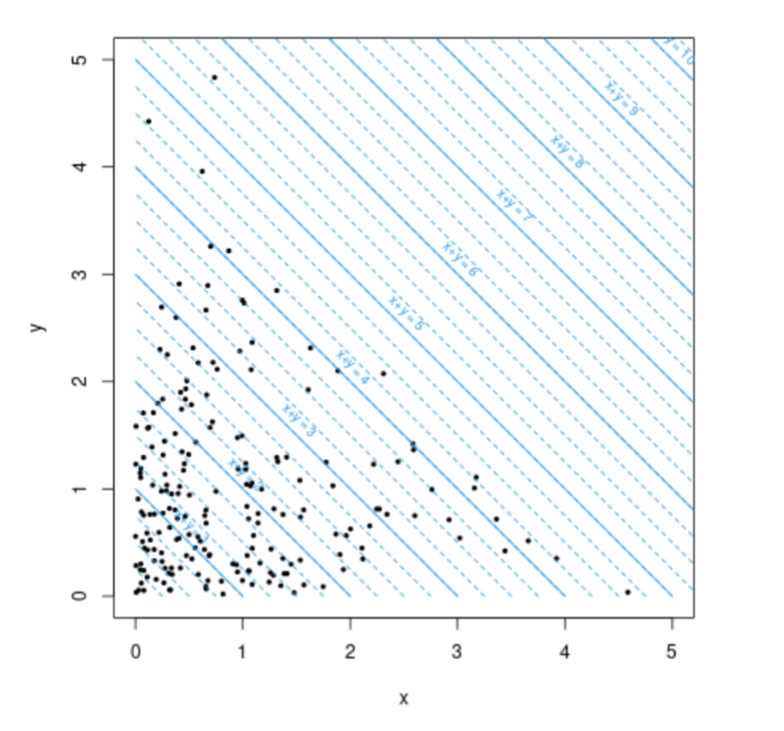
See the image below where 200 points are simulated where $X$ and $Y$ are independent exponential distributed.
You can see that the density is highest in the bottom left corner $X,Y = 0,0$
We have superimposed iso-lines for the sum $X+Y$. If you count between which iso-lines you find the most points is it between 0 and 0.25, or somewhere else?
The condition $X+Y = a$ covers a greater region in the joint distribution when $a$ is larger. That is what changes the distribution. It makes larger values more likely and smaller values less likely. The zero that had first infinite probability density has now zero probability density.
Chi square RVs are generally associated with distribution of variances whereas exponentially distributed RV is often associated with the probability of time until next event. So, how do we resolve these two seemingly different interpretations
Both interpretations relate to sums.
For the sum of two variables, their variance is the sum of the individual variances
For two subsequent waiting times, the total waiting time is the sum of the individual waiting times.
The relationship between the gamma distribution and the normal distribution

