2
$\begingroup$

I'm working on the forecasting of life expectancy actually. I have written code following the usual procedure. The results are not trustworthy because the life expectancy should have a positive slope (logically) but in my case it comes flat for the 50 years ahead. The ARIMA(1,1,2) is the best model with the lowest AICc. I'm in trouble with the point forecast where the straight line is flat. How do you think I can modify my code in order to get more powerful results enter image description here
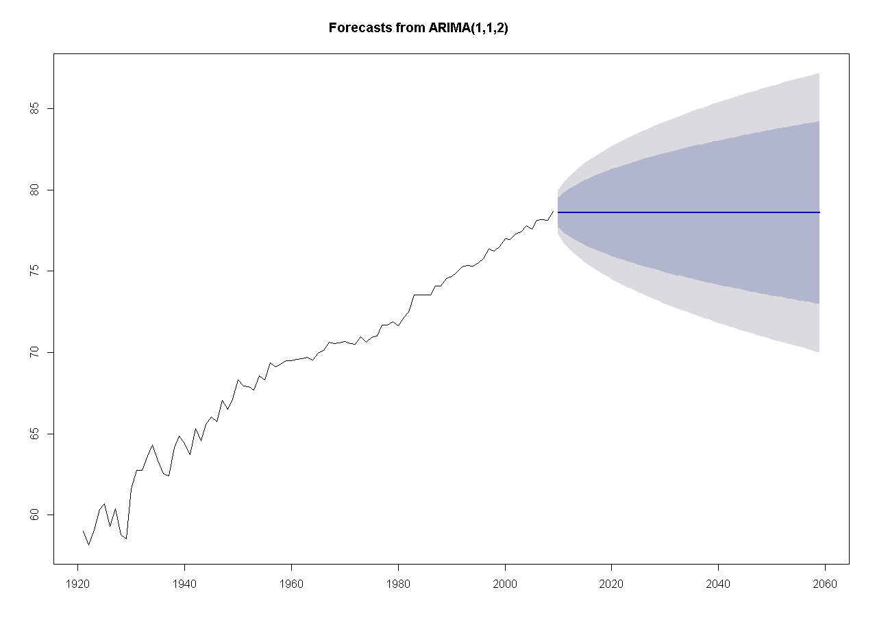
Here you find my code and the plot. The life expectancy is I(1). I have differenced it and the first difference is I(0). The first difference of life expectancy is stationary. Then I got the best model with the lowest AICc and forecast the the life expectancy level.

library(forecast)
AA<-Alberta$Male
AA1<-ts(AA,start=1921,end=2009,frequency=1)
A2<-diff(AA1,1)
fit1<-arima(A2, order=c(1,1,0))
fit2 <-arima(A2, order=c(1,1,1))
fit3<-arima(A2, order=c(1,1,2))
fit4<-arima(A2,order=c(2,1,0))
fit5<-arima(A2,order=c(2,1,1))
fit6<-arima(A2,order=c(2,1,2))
fit1
fit2
fit3
fit4
fit5
fit6
fit15<-arima(AA1,order=c(1,1,2))
ARIMA50ALBERTA<-forecast(fit15,50)
plot(ARIMA50ALBERTA)

These are the results:

 Point     Forecast    Lo 80    Hi 80    Lo 95    Hi 95
2010       78.63251 77.74617 79.51885 77.27697 79.98806
2011       78.59585 77.37187 79.81984 76.72393 80.46778
2012       78.61099 77.16457 80.05740 76.39888 80.82309
2013       78.60474 76.95134 80.25814 76.07608 81.13340
2014       78.60732 76.77553 80.43911 75.80584 81.40880
2015       78.60625 76.60992 80.60259 75.55312 81.65938
2016       78.60669 76.45917 80.75422 75.32234 81.89105
2017       78.60651 76.31746 80.89557 75.10570 82.10732
2018       78.60659 76.18437 81.02880 74.90213 82.31104
2019       78.60656 76.05809 81.15502 74.70901 82.50410
2020       78.60657 75.93783 81.27531 74.52509 82.68805
2021       78.60656 75.82274 81.39039 74.34907 82.86405
2022       78.60657 75.71223 81.50090 74.18006 83.03307
2023       78.60656 75.60578 81.60734 74.01727 83.19586
2024       78.60656 75.50299 81.71014 73.86006 83.35307
2025       78.60656 75.40349 81.80964 73.70789 83.50524
2026       78.60656 75.30699 81.90614 73.56030 83.65283
2027       78.60656 75.21323 81.99990 73.41691 83.79622
2028       78.60656 75.12200 82.09113 73.27738 83.93575
2029       78.60656 75.03309 82.18004 73.14141 84.07172
2030       78.60656 74.94635 82.26678 73.00874 84.20439
2031       78.60656 74.86161 82.35152 72.87915 84.33398
2032       78.60656 74.77874 82.43439 72.75242 84.46071
2033       78.60656 74.69764 82.51549 72.62838 84.58475
2034       78.60656 74.61818 82.59495 72.50686 84.70627
2035       78.60656 74.54027 82.67286 72.38771 84.82542
2036       78.60656 74.46383 82.74930 72.27080 84.94233
2037       78.60656 74.38878 82.82435 72.15602 85.05711
2038       78.60656 74.31504 82.89809 72.04324 85.16989
2039       78.60656 74.24254 82.97059 71.93236 85.28077
2040       78.60656 74.17123 83.04190 71.82330 85.38983
2041       78.60656 74.10104 83.11209 71.71596 85.49717
2042       78.60656 74.03193 83.18119 71.61027 85.60286
2043       78.60656 73.96386 83.24927 71.50615 85.70698
2044       78.60656 73.89676 83.31637 71.40354 85.80959
2045       78.60656 73.83061 83.38252 71.30237 85.91076
2046       78.60656 73.76536 83.44777 71.20258 86.01055
2047       78.60656 73.70098 83.51215 71.10412 86.10901
2048       78.60656 73.63743 83.57570 71.00694 86.20619
2049       78.60656 73.57469 83.63844 70.91098 86.30215
2050       78.60656 73.51272 83.70041 70.81620 86.39693
2051       78.60656 73.45149 83.76164 70.72256 86.49057
2052       78.60656 73.39098 83.82214 70.63002 86.58311
2053       78.60656 73.33117 83.88196 70.53855 86.67458
2054       78.60656 73.27203 83.94110 70.44810 86.76503
2055       78.60656 73.21353 83.99960 70.35864 86.85449
2056       78.60656 73.15567 84.05746 70.27014 86.94299
2057       78.60656 73.09841 84.11472 70.18257 87.03056
2058       78.60656 73.04174 84.17139 70.09590 87.11723
2059       78.60656 72.98564 84.22749 70.01010 87.20303
$\endgroup$
4
  • $\begingroup$ You've picked a bad model, so it isn't surprising the result looks bad. Try a different arima specification or an exponential smoothing model. $\endgroup$
    – Zach
    Commented Aug 26, 2013 at 22:21
  • 1
    $\begingroup$ You appear to have "drift" in your random walk component, but it doesn't sound like your model has a term for it. If your data has obvious features your model lacks, your model will tend to produce forecasts that are obviously lacking. $\endgroup$
    – Glen_b
    Commented Aug 26, 2013 at 22:27
  • 1
    $\begingroup$ I see two (perhaps non-obvious) ways to add a drift term using arima in R - one is to fit an ARIMA(1,0,2) to the differences, and another is to use the time index in the xreg argument. I'm not sure why they don't allow you to set include.mean=TRUE on an integrated model to fit the drift, but that's how it is. Some of the other packages/functions that fit time series probably allow it more directly. $\endgroup$
    – Glen_b
    Commented Aug 26, 2013 at 22:35
  • 1
    $\begingroup$ ... and I've only just noticed what you're forecasting. There are relatively widely used models for forecasting mortality curves (and hence, life expectancy) already, including some R packages. You might want to take a look at this as a starting point. There are numerous relevant papers and some books $\endgroup$
    – Glen_b
    Commented Aug 26, 2013 at 22:42

4 Answers 4

5
$\begingroup$

Try using auto.arima() instead of doing your own model search. I'm sure it will come up with a better model than the one you have. For a start, it will consider the inclusion of a drift term to allow for the trend in the data.

$\endgroup$
1
  • $\begingroup$ Thank you very for all your advises. It works very well! $\endgroup$ Commented Aug 27, 2013 at 19:53
0
$\begingroup$

I think that the issue might be explained in the following link : ISSUE 3: Why does predict.Arima give strange forecasts? in the Nevertheless, the author uses the predict function instead of forecast. However, the issue seem to be really alike to the explained here, having a straight line in the forecast

Copy from the link:

If you want to get predictions from an ARIMA(p,d,q) fit when there is differencing (i.e., d > 0), then the previous issue continues to be a problem. Here's an example using the global temperature data from Chapter 3. In what you'll see below, the first method gives the wrong results and the second method gives the correct results. I think it's just best to stay away from the first method. If you use sarima and sarima.for, then you'll avoid these problems.

 u=read.table("/mydata/globtemp2.dat")  # read the data
 gtemp=ts(u[,2],start=1880,freq=1)      # yearly temp in col 2
 fit1=arima(gtemp, order=c(1,1,1))   
 fore1=predict(fit1, 15)   
 nobs=length(gtemp)                
 fit2=arima(gtemp, order=c(1,1,1), xreg=1:nobs)  
 fore2=predict(fit2, 15, newxreg=(nobs+1):(nobs+15))
 par(mfrow=c(2,1))
 ts.plot(gtemp,fore1$pred,col=1:2,main="WRONG")
 ts.plot(gtemp,fore2$pred,col=1:2,main="RIGHT")

I hope that it is useful for someone.

$\endgroup$
1
  • $\begingroup$ Best not to have your answer rely on linked information, as links do break over time. If you could abstract the key points made in the link and incorporate them into your answer, that would be much better! $\endgroup$
    – jbowman
    Commented Jan 3, 2019 at 18:40
0
$\begingroup$

Visually it appears to have multiple drifts and multiple changes in either error variance or model parameters ...Only your data knows for sure . Forcing the data into a pre-set of models can have serious consequences. Post the actual data and I will try and help further .

$\endgroup$
0
$\begingroup$

the life expectancy should have a positive slope (logically)

Why should life expectancy have a positive slope, logically? Even if it's positive, why should it be constant?

Here's what Canadian actuary has to say:

Jean-Claude Ménard, Canada's Chief Actuary, said the improvement in life spans is not projected to continue at the same rate into the future. His office's projections assume the pace of gains will continue for the next few years, then gradually slow.

I'd argue that the forecast you made (mistakenly, accidentally) is better than any "proper, correct" time time series forecast will produce. The reason being is that the time series forecast will pick up the trend and continue it into future in some shape or form. It doesn't have to do it by primitive trend extraction, it can be done in a very sophisticated manner, but in the end it will pick up the growth trend.

I'm going to say that Alberta Male life expectancy will not keep growing at the historical pace anymore. 80 years is an excellent guess for the future, it's not going to be 85 by 2040.

$\endgroup$
3
  • $\begingroup$ the "trend" can be abated by recent data ...thus while globally there may be a strong upwards trend recent values may not support that thus possible abatement to diminish the estimated trend. Analytically detecting the changes in trends is a particular "hobby" of mine . Consider a series 1,2,3,...100,100,100,100,100,100 even with some random variation superimposed can yield a change point given that the "random variation" is small enough.. $\endgroup$
    – IrishStat
    Commented Jan 3, 2019 at 16:28
  • $\begingroup$ @IrishStat, if anything, the latest data in OP's series would not show you any hints of slower growth of life expectancy. My argument is that pure time series modeling will not work for long term forecast $\endgroup$
    – Aksakal
    Commented Jan 3, 2019 at 16:31
  • $\begingroup$ agreed ... I was just trying to reflect that changes in trends can sometimes be detected and should be tested for . $\endgroup$
    – IrishStat
    Commented Jan 3, 2019 at 20:12

Your Answer

By clicking “Post Your Answer”, you agree to our terms of service and acknowledge you have read our privacy policy.

Not the answer you're looking for? Browse other questions tagged or ask your own question.