3
$\begingroup$

I have a question about how to tell two different mixed effects models apart. In the simple case both involve fitting a model with a random group effect and a covariate. I fit the model with lme4 in R. Here is a visualization of the two different scenarios.
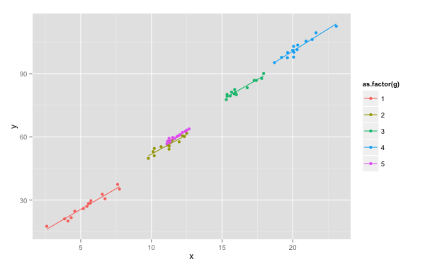
enter image description here

library(ggplot2)
library(lme4)
gen_dat2 <- function(group.m,group.v,int, sl,n){
      x <- vector()
      y <- vector()
      g <- vector()
         for(i in 1:length(group.m)){
         x.t <- rnorm(n,group.m[i],group.v[i])
         y.t <- rnorm(n,group.m[i],group.v[i])+int + sl*x.t 
         x <- c(x,x.t)
         y <- c(y,y.t)
         g <- c(g,rep(i,n))
        }
     return(cbind(x,y,g))
}

group.m <- runif(5,1,20)
group.v <- runif(5,1,1.5)

dat2 <- data.frame(gen_dat2(group.m,group.v,1,4,14))
ggplot(dat2,aes(x=x,y=y,colour=as.factor(g),group=g))+geom_point()+stat_smooth(method="lm",se=F)
m2 <- lmer(y~x + (x|g),data=dat2)

Then I can generate and fit the other scenario with similar code:
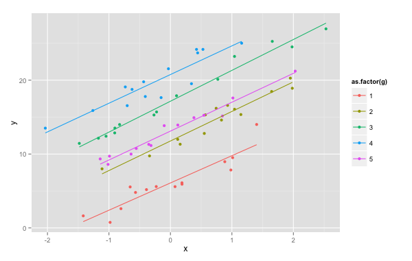
enter image description here

 gen_dat <- function(group.m,group.v,int, sl,n){
      x <- vector()
      y <- vector()
      g <- vector()
         for(i in 1:length(group.m)){
         x.t <- rnorm(n,0,1)
         y.t <- rnorm(n,group.m[i],group.v[i])+int + sl*x.t 
         x <- c(x,x.t)
         y <- c(y,y.t)
         g <- c(g,rep(i,n))
        }
     return(cbind(x,y,g))
}

group.m <- runif(5,1,20)
group.v <- runif(5,1,1.5)

dat1 <- data.frame(gen_dat(group.m,group.v,1,4,14))
ggplot(dat1,aes(x=x,y=y,colour=as.factor(g),group=g))+geom_point()+stat_smooth(method="lm",se=F)
m1 <- lmer(y~x + (x|g),data=dat1)

My central question is how do I tell these two models apart? Am I incorrectly fitting the first one, and I need an extra term in there to model the relationships between groups and the x variable as well as y? Both detect substantial between group variation in the intercept and not much in the slope as I would predict. But I need a way to tell these two apart. Any thoughts would be helpful.


Edits:

This has been helpful in me restating the question. So I want to re-ask the question with an example which I hope will make it clear why I want to be able to tell these two models apart. Let's imagine that Y is the average student test score at a school, and X is spending per student in that school. Our grouping variables are 5 different school districts.

Data in the top figure shows that an increase in spending within a district means that test scores increase. It also shows that between districts there are differences is scores, but that's clearly because some districts spend more student than others.

Data in the second figure show similarly that within a district student scores increase as spending increases. It also shows that between districts there are differences in test scores. However we don't know what is driving those differences, unlike in the first set of data. This is a pretty common situation I've encountered in building models. The former is not.

So what I'm asking is what is the appropriate model that captures the following features from the first dataset:

  1. Test scores increase as spending per student does
  2. There is also variance between districts in student test scores
  3. Part of that difference between districts is because of the underlying relationship between spending and test scores, which also varies with district.

More generally stated, how do you handle a scenario where you're building a hierarchical model where the grouping variable is correlated with one of your continuous independent variables (e.g. the first scenario). I feel like the model I've presented get's at points 1. and 2., but not point 3. So I'm really seeking a way to tease these two scenarios apart.

Normally I might add an extra level of hierarchy if there was another group level explanatory variable. Continuing our example, maybe in the 2nd dataset there are differences between district because in some districts parents have more time to spend on homework with students. So we would add that as a group level predictor in a hierarchical model. But that wouldn't work in the first scenario.

$\endgroup$
6
  • 1
    $\begingroup$ I don't understand what you mean about telling the models apart. They have different coefficients. They have different variances in the random effects. So they're different. I'm not sure what I'm missing. $\endgroup$ Commented Oct 11, 2013 at 0:02
  • $\begingroup$ In addition to David's comment for extra clarifications. While I really appreciate the fact you went into the trouble of giving R-code unless you specify the random seed (eg. set.seed(0)) one will not be able to replicate your results/graphs. (In general, code comments would be a plus too.) $\endgroup$
    – usεr11852
    Commented Oct 11, 2013 at 0:20
  • $\begingroup$ @DavidJ.Harris True, but I feel like I'm not fitting the right model in the first scenario. I don't think it's the right model in the first scenario, because intuitively, all those lines seem to have the same slope and the same intercept. So I guess I'm wondering, what's the 3rd parameter that says "There's variation between groups in the slope, the intercept and the x-values of the groups". Perhaps my question is more, is there a better model to answer the preceding question? $\endgroup$
    – emhart
    Commented Oct 11, 2013 at 0:39
  • $\begingroup$ If you want all the differently-colored groups to have the same slopes and same intercepts, then you can enforce that by removing the random effect. $\endgroup$ Commented Oct 11, 2013 at 0:43
  • 3
    $\begingroup$ In general, linear regression techniques don't have much to say about $x$, just about $y|x$. There's nothing in either model that says orange has to be on the left and blue has to be on the right. $\endgroup$ Commented Oct 11, 2013 at 0:44

1 Answer 1

2
$\begingroup$

You don't need extra terms in the models, less actually. It is plain to see by your plots, but if you look at summary(m2) you will see that the variance for random effect for x is really small, and the variance for the intercept is quite small as well.

Similarly for the m1 model, you can see from the plot that the slopes are all the same, but the intercept varies. You can use an F-test to check the model with only random intercepts versus the model with random slopes and intercepts you specified.

m1 <- lmer(y~x + (x|g),data=dat1)
m1RInt <- lmer(y~x + (1|g),data=dat1)
anova(m1,m1RInt)

Also just looking at the variance estimates of the random intercepts and effects for summary(m1) you would have come to the same conclusion that using random slopes adds nothing to the model.

$\endgroup$
8
  • $\begingroup$ This has been helpful in me restating the question. What I'm getting at is how could I tell apart the following scenarios. $\endgroup$
    – emhart
    Commented Oct 11, 2013 at 16:29
  • $\begingroup$ @DistribEcology, are you asking about whether x significantly varies between g? That might be best answered by boxplots of x ~ g or an anova. If you are asking about whether x has a differing effect in different g, then you can use the example in my answer as an inferential test between the models (one with random effects and random intercepts and one with only a random intercept). $\endgroup$
    – Andy W
    Commented Oct 11, 2013 at 17:09
  • $\begingroup$ I tried to elucidate the question by adding significant edits to the question, which maybe you can check out. But I'm not sure I follow that adding random intercepts adds nothing. Do you mean slopes? Clearly there's lot's of variance between intercepts, but none between slopes. $\endgroup$
    – emhart
    Commented Oct 11, 2013 at 17:18
  • 1
    $\begingroup$ Like David said in the comment, it seems your asking about the between group variation for x within g, which doesn't have anything to do with a model of y = x|g. x varying within g is neither a necessary nor sufficient condition for intercepts or slopes to vary when predicting y. So a second test seems appropriate to answer that question - although your example graphic sort of says it all in this example. $\endgroup$
    – Andy W
    Commented Oct 11, 2013 at 17:30
  • 1
    $\begingroup$ You can evaluate whether "Part of that difference between districts is because of the underlying relationship between spending and test scores" by seeing how much of the variance associated with your district grouping factor disappears when you remove (or randomize) spending. $\endgroup$ Commented Oct 11, 2013 at 18:46

Your Answer

By clicking “Post Your Answer”, you agree to our terms of service and acknowledge you have read our privacy policy.

Not the answer you're looking for? Browse other questions tagged or ask your own question.