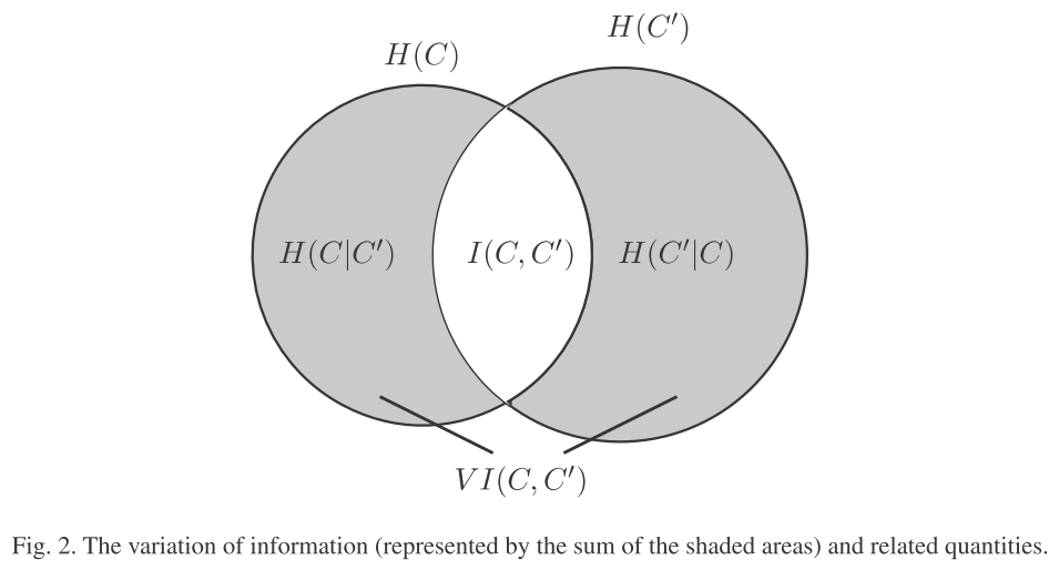
For non-statisticians like me, it is very difficult to capture the idea of VI metric (variation of information) even after reading the relevant paper by Marina Melia "Comparing clusterings - An information based distance" (Journal of Multivariate Analysis, 2007). In fact, I am not familiar with many of the clusterings' terms out there.
Below is a MWE and I would like to know what does the output mean in the different metrics used. I have these two clusters in R and in the same order of id:
> dput(a)
structure(c(4L, 3L, 4L, 4L, 4L, 4L, 4L, 3L, 4L, 4L, 3L, 3L, 3L,
4L, 4L, 4L, 4L, 4L, 3L, 4L, 4L, 4L, 3L, 4L, 4L, 3L, 4L, 4L, 4L,
1L, 1L, 4L, 4L, 4L, 4L, 4L, 4L, 3L, 4L, 4L, 3L, 4L, 4L, 2L, 2L,
4L, 3L, 3L, 2L, 2L, 2L, 4L, 3L, 4L, 4L, 3L, 1L, 4L, 3L, 4L, 4L,
4L, 3L, 4L, 4L, 4L, 4L, 2L, 2L, 2L, 4L, 3L, 4L, 4L, 4L, 4L, 4L,
4L, 4L, 4L, 4L, 3L, 4L, 4L, 3L, 4L, 4L, 4L, 4L, 4L, 4L, 3L, 4L,
4L, 3L, 4L, 4L, 4L, 4L, 4L, 4L, 3L, 4L, 4L, 4L, 4L, 2L, 2L, 4L
), .Label = c("1", "2", "3", "4"), class = "factor")
> dput(b)
structure(c(4L, 3L, 4L, 4L, 4L, 4L, 4L, 3L, 4L, 4L, 3L, 3L, 3L,
4L, 4L, 3L, 4L, 4L, 3L, 4L, 4L, 4L, 3L, 4L, 4L, 3L, 4L, 4L, 4L,
1L, 1L, 4L, 4L, 4L, 4L, 4L, 4L, 3L, 4L, 4L, 3L, 4L, 4L, 2L, 2L,
4L, 3L, 3L, 2L, 2L, 2L, 4L, 3L, 4L, 4L, 3L, 1L, 4L, 3L, 4L, 4L,
3L, 3L, 4L, 4L, 4L, 4L, 2L, 2L, 2L, 4L, 3L, 3L, 4L, 4L, 4L, 4L,
4L, 4L, 4L, 4L, 3L, 4L, 4L, 3L, 4L, 4L, 4L, 4L, 4L, 4L, 3L, 4L,
4L, 3L, 4L, 4L, 4L, 4L, 4L, 3L, 3L, 4L, 4L, 4L, 4L, 2L, 2L, 4L
), .Label = c("1", "2", "3", "4"), class = "factor")
Now doing comparisons based on the VI as well as other metrics / indices and in chronological order of their appearance in literature.
library(igraph)
  # Normalized Mutual Information (NMI) measure 2005:
compare(a, b, method = c("nmi"))
[1] 0.8673525
  # Variation of Information (VI) metric 2003:
compare(a, b, method = c("vi"))
[1] 0.2451685
  # Jaccard Index 2002:
clusteval::cluster_similarity(a, b, similarity = c("jaccard"), method = "independence")
[1] 0.8800522
  # van Dongen S metric 2000:
compare(a, b, method = c("split.join"))
[1] 8
  # Adjusted Rand Index 1985:
compare(a, b, method = c("adjusted.rand"))
[1] 0.8750403
  # Rand Index 1971:
compare(a, b, method = c("rand"))
[1] 0.9374788
As you can see, the VI value was different from all the others.
- What does this value tell (and how is it related to the figure below)?
- What are the guidelines for considering this value low or high?
- Are there any guidelines defined?
Maybe experts in the field can provide some sensible descriptions for laymen like me when trying to report such results. I would really appreciate if someone would provide also guidelines for other metrics as well (when to consider the value is large or small, i.e., in relation to a similarity between two clusters).
I have read related CV threads here and here, but still couldn't grasp the intuition behind VI. Can someone explain this in plain English?
The below figure is figure 2 from the above mentioned paper about VI.

