Your understanding looks correct, but when talking to statisticians it's best not to use the word 'likelihood' when you mean 'probability'; in statistics likelihood is a technical term with a very specific meaning (one that isn't the same thing as probability).
When computing sample size, it's common to specify what power is desired for a specific effect size (for some situations, a few additional details or assumptions may be required as well).
If you specify a minimum desired power at a given a sample size, then the effect size that gives that power is often called the "minimum detectable difference".
If the true effect size is larger, the power will be larger (just as you said), if it's smaller, the power will be smaller.
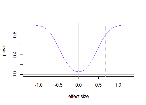
If you draw the relationship between power and effect size, you get a thing called a power curve.
Here's a power curve for a two-sample t-test, n=35 in each group, with the effect size measured in number of $\sigma$'s of difference between means:

The 80% power line is marked in, and corresponds to an effect size of about $0.68\sigma$. In this case both sides of the power curve are shown, but for symmetric cases it's common to omit the left side (or equivalently to put the effect size as $|\mu_1-\mu_2|/\sigma$, thus only getting the curve on right side in the above diagram).
The "power" at effect size 0 is really the probability of rejection when the null is true (i.e. not actually power at that point) - which is of course the significance level, $\alpha$; in the above plot that's 0.05. Normally the rejection rate at that point is drawn in, even though it's not strictly power.
Here are a few other examples of power curves (used in answers to other questions):
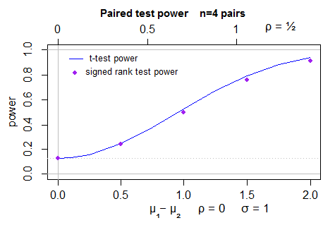
(1) A power comparison of paired t-test (curve) and Signed Rank test (points) for 4 pairs of normal observations (it's actually two-sided, but the left half isn't shown as it's a mirror image of the right half):

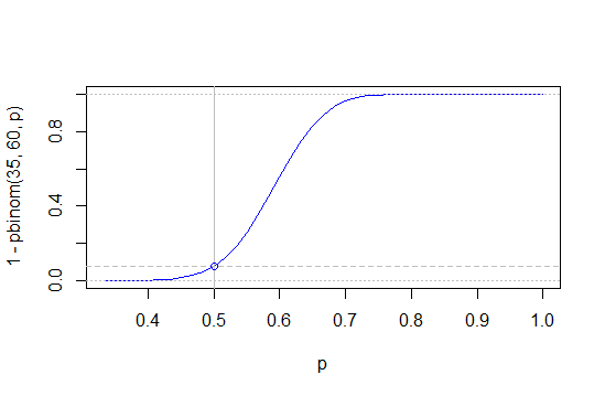
(2) Power for a binomial (one tailed test):

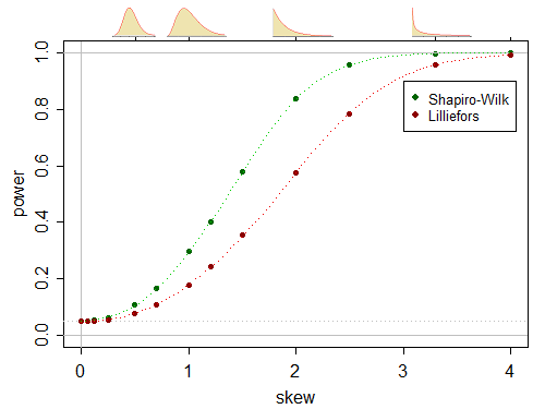
(3) These can even be drawn for goodness of fit tests if you restrict consideration to a particular set of alternatives (in this case, the null is normality, and the subset of alternatives considered in this power comparison are gamma distributions):
