Return to Revisions

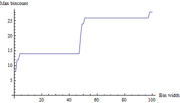
You could divide the data into equal bins to find the bin size (and offset) that yields a suitable maximum bin count. Here is an example using the following data.

a = {463, 463, 512, 512, 512, 512, 512, 512, 512,
     512, 513, 513, 513, 513, 10462, 10462, 880, 880,
     929, 929, 929, 929, 929, 929, 929, 929, 930, 930,
     930, 930, 10879, 10879, 181, 181, 230, 230, 230, 
     230, 230, 230, 230, 230, 231, 231, 231, 231, 10180,
     10180, 416, 416, 465, 465, 465, 465, 465, 465, 465,
     465, 466, 466, 466, 466, 10415, 10415};

maxA = 10415;

Increasing the bin count from 1 to 100 (offsetting the bin start to capture all variations) produces the following plot of maximum bin count. For example, a bin size of 4 with an offset of 3 captures a maximum bin count of 14, and a bin size of 48 with an offset of 33 captures a maximum bin count of 20.

Selecting from a where (33 + 48 * 9) <= a < (33 + 48 * 10) finds 20 items.

Mathematica code for the above

largestBinWidth = 100;

counts = Table[
   Table[
    {binsize, offset, 
     Max[BinCounts[a, {offset, maxA + offset, binsize}]]},
    {offset, -binsize, binsize}],
   {binsize, 1, largestBinWidth}];

maxcounts = Last[SortBy[#, Last]] & /@ counts;

ListLinePlot[maxcounts[[All, {1, 3}]],
 PlotRange -> All, AxesOrigin -> {0, 0},
 AxesLabel -> {"Bin width", "Max bincount"}]