I believe there may be a Bayesian-style approach to get the equations given in the paper's appendix B.
As I understand it, the experiment boils down to a statistic $z\sim\mathrm{N}_{\theta,1}$. The mean $\theta$ of the sampling distribution is unknown, but vanishes under the null hypothesis, $\theta\mid{}H_0=0$.
Call the experimentally observed statistic $\hat{z}\mid\theta\sim\mathrm{N}_{\theta,1}$. Then if we assume a "uniform" (improper) prior on $\theta\sim1$, the Bayesian posterior is $\theta\mid\hat{z}\sim\mathrm{N}_{\hat{z},1}$. If we then update the original sampling distribution by marginalizing over $\theta\mid\hat{z}$, the posterior becomes $z\mid\hat{z}\sim\mathrm{N}_{\hat{z},2}$. (The doubled variance is due to convolution of Gaussians.)
Mathematically at least, this seems to work. And it explains how the $\frac{1}{\sqrt{2}}$ factor "magically" appears going from equation B2 to equation B3.
Summary: The trick appears to be a Bayesian approach which assumes a uniform (Jeffreys) prior for the hidden parameter ($z_\mu$ in appendix B of the paper, $\theta$ here).
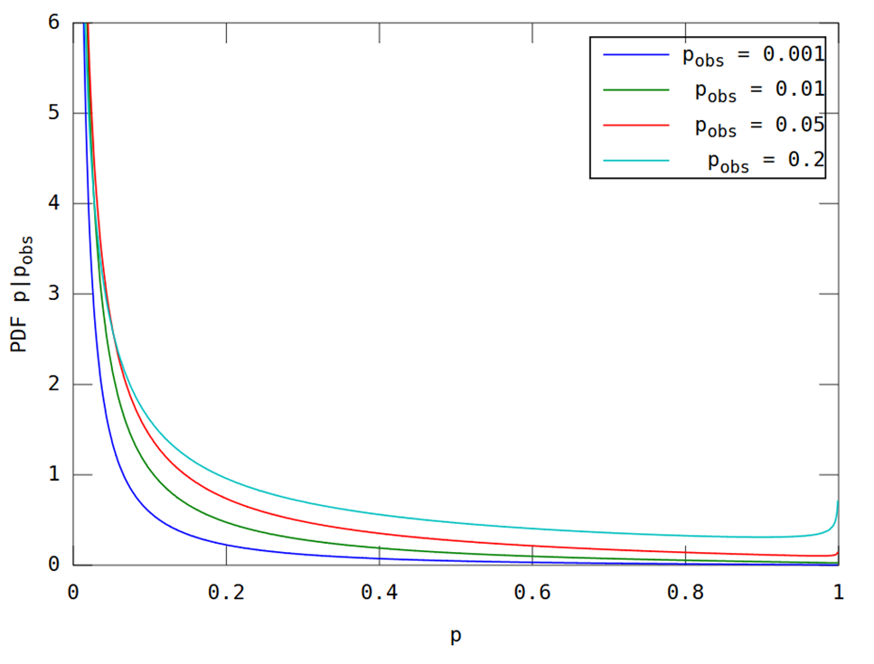
As requested in the comments, here is a plot for comparison. This is a relatively straightforward application of the formulas in the paper. However I will write these out to ensure no ambiguity.
Let $p$ denote the one-sided p value for the statistic $z$, and denote its (posterior) CDF by $F[u]\equiv\Pr\big[\,p\leq{u}\mid{\hat{z}}\,\big]$. Then equation B3 from the appendix is equivalent to $$F[p]=1-\Phi\left[\tfrac{1}{\sqrt{2}}\left(z[p]-\hat{z}\right)\right] \,,\, z[p]=\Phi^{-1}[1-p]$$ where $\Phi[\,\,]$ is the standard normal CDF. The corresponding density is then $$f\big[p\big]\equiv{F^\prime}\big[p\big]=\frac{\phi\Big[(z-\hat{z})/\sqrt{2}\,\Big]}{\sqrt{2}\,\phi\big[z\big]}$$ where $\phi[\,\,]$ is the standard normal PDF, and $z=z[p]$ as in the CDF formula. Finally, if we denote by $\hat{p}$ the observed two-sided p value corresponding to $\hat{z}$, then we have $$\hat{z}=\Phi^{-1}\Big[1-\tfrac{\hat{p}}{2}\Big]$$
Using these equations gives the figure below, which should be comparable to the paper's figure 5 quoted in the question.

(This was produced by the following Matlab code; run here.)
phat2=[1e-3,1e-2,5e-2,0.2]'; zhat=norminv(1-phat2/2);
np=1e3+1; p1=(1:np)/(np+1); z=norminv(1-p1);
p1pdf=normpdf((z-zhat)/sqrt(2))./(sqrt(2)*normpdf(z));
plot(p1,p1pdf,'LineWidth',1); axis([0,1,0,6]);
xlabel('p'); ylabel('PDF p|p_{obs}');
legend(arrayfun(@(p)sprintf('p_{obs} = %g',p),phat2,'uni',0));
