I have two random variables $s\sim \mathcal{N}(\nu,\sigma)$ and $a\sim \mathcal{U}(0,A)$, $0<A<1$, calculate a third r.v. $t=(1-a)/s$ and want to find its distribution $p(t|\nu,\sigma,A)$.
My reasoning is, that for any value of $a$, there is exactly one $s=(1-a)/t$ such that the $(a,s)$ pair will produce $t$ and I will therefore have to integrate over the probabilities for these values:
$$p(t|\nu,\sigma,A) = \int_0^A p_a(x)p_s((1-x)/t)\,\mathrm dx\\$$
which can be expressed as the sum of two error functions.
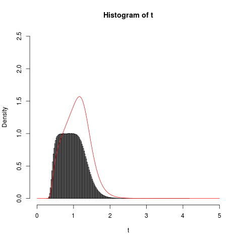
But already when checking this step numerically, I get a discrepancy between estimated (by sampling) and calculated distribution:

*Why do the histogram and the calculated distribution do not match?*
This is the code I used:
n=10000000
A=0.7
nu=.7
sigma=.1
# sampling from the target distribution
s=rnorm( n, mean=nu, sd=sigma )
a=runif( n, min=0, max=A )
t=(1-a)/s
hist(t,200, freq=F, xlim=c(0,5), ylim=c(0,2.5))
# plot the analytical result
analytic <- function(t, A, nu, sigma ){
tmp <- function(x, A, t, nu, sigma){
return (1/A*dnorm( (1-x)/t, mean=nu, sd=sigma) )
}
return( integrate( tmp, 0, A, A=A, t=t, nu=nu, sigma=sigma)$value)
}
x=seq(0,5,by=.01)
y=rep(0,length(x))
for( i in seq(1,length(x)) ){
y[i]=analytic(x[i], A, nu, sigma)
}
lines( x, y, col="red", type="l")