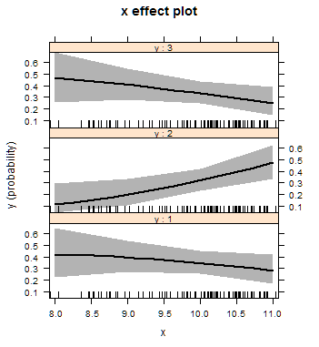
You can accomplish this with the `effects` package. Now, for a reproducible example:
library(nnet)
set.seed(892)
x <- c(rnorm(100, 10, 1))
y <- factor(rep_len(1:3, 100))
fit <- multinom(y ~ x)
That's the model, now let's get some predicted probabilities.
fit.eff <- Effect("x", fit)
data.frame(fit.eff$model.matrix, fit.eff$prob, fit.eff$lower.prob,
fit.eff$upper.prob)
X.Intercept. x prob.X1 prob.X2 prob.X3 L.prob.X1 L.prob.X2 L.prob.X3 U.prob.X1 U.prob.X2 U.prob.X3
1 1 8 0.4211010 0.1119309 0.4669680 0.2218766 0.03696574 0.2565056 0.6498212 0.2927143 0.6898823
2 1 9 0.3962450 0.1958841 0.4078709 0.2704241 0.10428467 0.2805946 0.5374796 0.3376147 0.5488354
3 1 10 0.3478412 0.3198070 0.3323518 0.2583849 0.23216366 0.2442887 0.4494968 0.4223378 0.4339321
4 1 11 0.2780225 0.4753991 0.2465784 0.1689652 0.33171768 0.1449846 0.4217471 0.6232722 0.3871286
Which gives the probabilities for factor "1" in X, `prob.X1`, its lower confidence interval `L.prob.X1` and its upper interval `U.prob.X1`.
`effects` will helpfully plot the values for you as well, which is its main purpose anyway.
plot(fit.eff)

Edit: added some code to clarify which levels of `x` were being predicted. Note that `Effect()` automatically cuts numerical predictor variables based on `grid.pretty`, which might not be what you typically want. In this case, you need to set the `xlevels` option, like this: `fit.eff <- effect("x", fit, xlevels = list(x = c(2, 4, 6, 8, 10)))`.