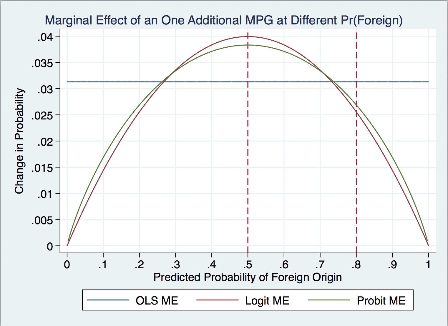
They are evaluating the average marginal effects at the two levels of probability. It's just the logit or probit coefficient times the derivative of the conditional probability for that model. You can do this with lincom or margins of an expression in Stata.
This is an old fashioned approach to showing marginal effects that was more popular when statistical software was less developed.
Edit:
In response your comment, here is some code showing the basic calculation using lincom on the cars dataset. I think you are mistaken about what these commands can accomplish. You can find the derivation of the marginal effect for logit here and probit here. There is some code at the end showing how to calculate the average marginal effects, which should have correct SEs and also will handle categorical variables correctly, and are arguably more representative that the approach in your paper.
#delimit;
sysuse auto, clear;

/* OLS */
regress foreign c.mpg, robust;
margins, dydx(mpg);

/* Logit MEs at p = 0.5 and p = 0.8 */
logit foreign c.mpg, nolog;
/* NB: these SEs are too small */
lincom .5*(1-.5)*_b[mpg];
lincom .8*(1-.8)*_b[mpg];

/* Probit MEs at p = 0.5 and p = 0.8 */
probit foreign c.mpg, nolog;
/* NB: these SEs are too small */
lincom `=normalden(invnormal(.5))'*_b[mpg];
lincom `=normalden(invnormal(.8))'*_b[mpg];

/* Plot for all possible values of p (not just 0.5 and 0.8) */
tw
    (function y = .0312915)
    (function y = x*(1-x)*.1597621, range(0 1))
    (function y = normalden(invnormal(x))*.0960601, range(0 1))
, ylab(#10, angle(horizontal) grid)
ytitle("Change in Probability")
xlab(#10, grid)
xtitle("Predicted Probability of Foreign Origin")
xline(.5 .8, lpatter(dash))
title("Marginal Effect of an One Additional MPG at Different Pr(Foreign)", span size(medium))
legend(label(1 "OLS ME" ) label(2 "Logit ME") label(3 "Probit ME") rows(1));


/* Average Marginal Effects with continuous and categorical covariates */
gen high_mpg = mpg>21;
logit foreign c.weight i.high_mpg, nolog;
margins, dydx(*);
The general plot looks like this, which shows that the effect depends on the baseline probability for logit and probit, but not for OLS, where the ME is constant. That is, the effect is biggest for observations near 1/2 and smallest in the very likely and very unlikely tails in non-OLS models:

