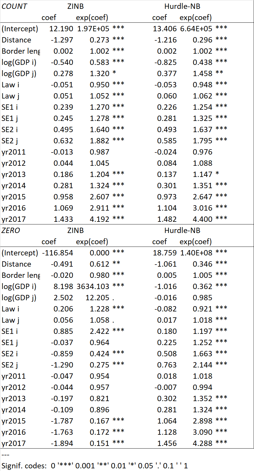
Below are a set of results from a zero-inflated (AIC = 64992.15; BIC = 65280.78) and hurdle model (AIC = 65141.73; BIC = 65430.36) for a dataset (>18000 obs) which describes the number of illicit firearms being purchased in one state and recovered by law enforcement in another. Using variables for each state (e.g. GDP, restrictive firearm laws, distance between states, and whether or not the states share a border and its length) I want to test whether positive counts of illicit weapon flows (F) and zero F are affected by such variables, and the level of influence each year between 2010 and 2017.

From what I've read so far, it seems like I should interpret from the ZINB that, when F = 0, for every increase in distance between states the odds of seeing zero F decreases by 61%. This part makes me think I'm interpreting it completely wrong, I was originally assuming that a greater distance would influence the F to drop, and now I'm in need of some guidance on how to read the model.

library(pscl)
zinb <- zeroinfl(Y ~ lCTD + BL + lGDPi + lGDPj + LIi + LIj + SE1i+ SE1j + SE2i + SE2j + yr, 
             data = modeldata, 
             dist = "negbin")
hdnb <- hurdle(Y ~ lCTD + BL + lGDPi + lGDPj + LIi + LIj + SE1i+ SE1j + SE2i + SE2j + yr, 
            dist = "negbin", 
            zero.dist = "binomial", 
            data = modeldata)


AIC(zinb, hdnb)
BIC(zinb, hdnb)

summary(zinb)
summary(hdnb)

fm <- list("ZINB" = zinb, "Hurdle-NB" = hdnb)
t(sapply(fm[1:2], function(x) round(x$coefficients$count, digits = 3)))
t(sapply(fm[1:2], function(x) round(exp(x$coefficients$count), digits = 3)))

library(countreg)
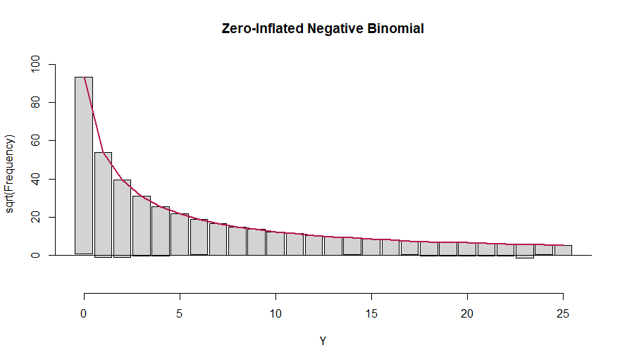
rootogram(zinb, main = "Zero-Inflated Negative Binomial", ylim = c(-15, 100), max = 25)
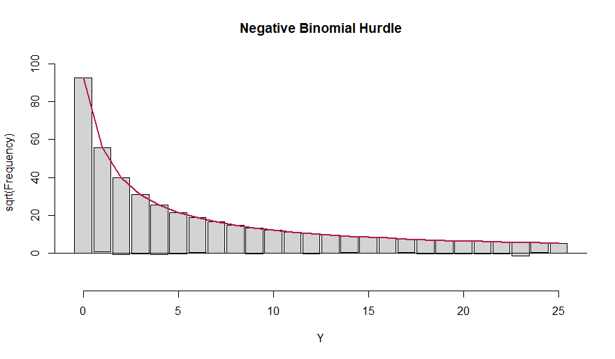
rootogram(hdnb, main = "Negative Binomial Hurdle", ylim = c(-15, 100), max = 25)
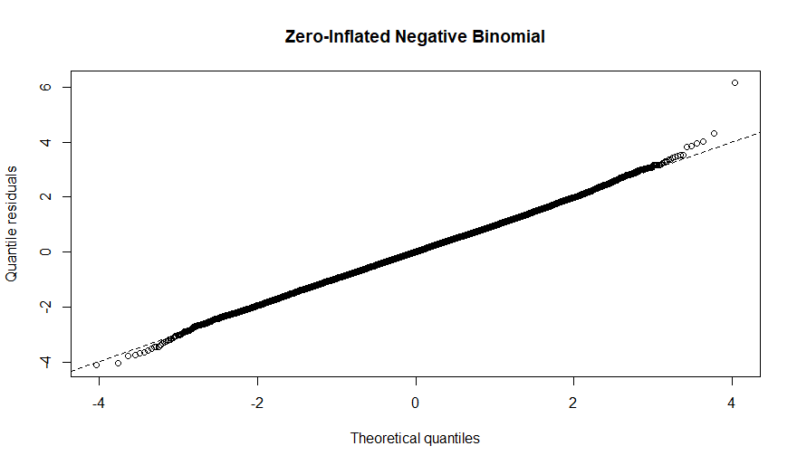
qqrplot(zinb, main = "Zero-Inflated Negative Binomial")
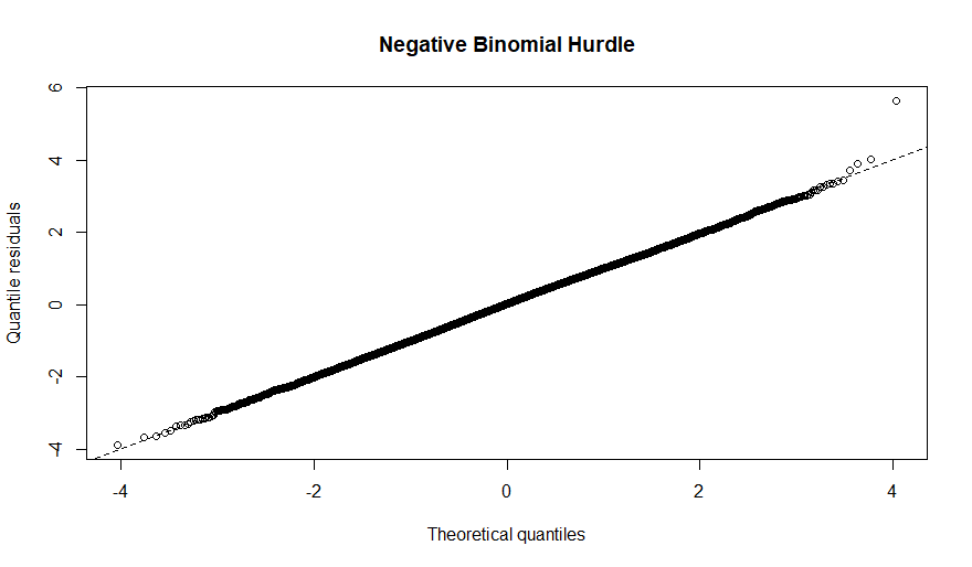
qqrplot(hdnb, main = "Negative Binomial Hurdle")