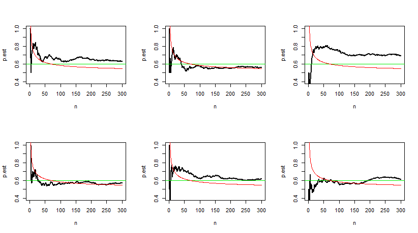
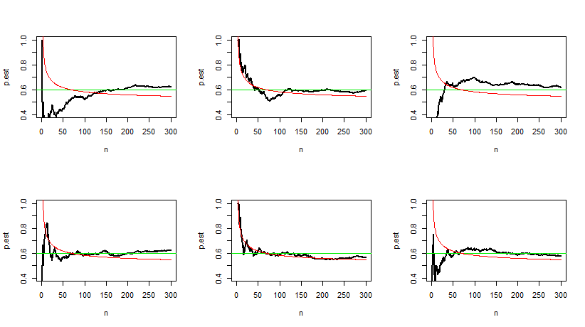
This is to illustrate how undesigned early stopping may be unwise, as mentioned in @rishi-k's comment.
Suppose you have binomial data and are testing hypotheses about Success probability $p.$ In particular, consider testing $H_0: p = 0.5$ against $H_a: p > 0.5$ at the 5% level.
In order to get good power against the specific alternative $p = 0.6$ you will
need about $n = 300$ Bernoulli observations. As shown by the following
simulation, using the exact binomial test implement in the R procedure binom.test. [You will get about the same required sample size using an
approximate normal test. Perhaps see formulas here.]
set.seed(1103)
pv =  replicate(10^5,
       binom.test(rbinom(1,300,.6),300,,alt="gr")$p.val)
mean(pv <= .05)
[1] 0.9659     # aprx power
Now let's look at traces of twelve experiments at each step 1, 2, ..., 300. The jagged black curves show the estimated Success probability $\hat p = X_i/i,$ for $i = 1, 2, \dots, 300.$ The red curves show critical values of the approximate normal test at each step, which are computed according to $H_0.$ Asymptotically, they approach $0.5.$
It is clear that by the time we have 300 observations (at the right of each panel) the jagged black curve (trending towards $0.6)$ is very likely to have risen above the (red) critical value.
However, in several of the twelve panels the first crossing of the black trace above the critical value occurs substantially before 300 observations have been collected. If we were to stop at the first crossing we would not have an honest conclusion.
Sequential analysis allows for early stopping, but for legitimate early stopping the red curves have to be different (harder to cross).
Note: Here is R code for the figures. The last six runs were made using the seed shown.
set.seed(2021)
par(mfrow=c(2,3))
 for(i in 1:6){
  N=300; n = 1:N
  x = rbinom(N, 1, .6)
  p.est = cumsum(x)/n
  plot(n, p.est, ylim=c(.4,1), lwd=2,type="l")
   abline(h=.6, col="green2")
   upr = 1/2 + (1.645/2)/sqrt(n)
   lines(n, upr, col="red")
  }
par(mfrow=c(1,1))


