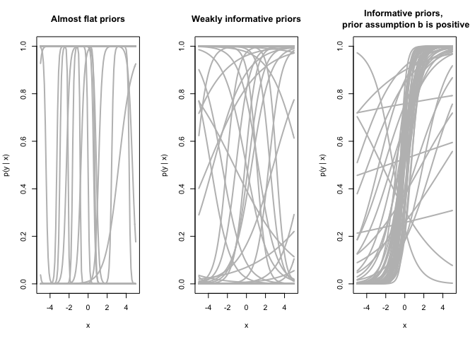
One trick is to simulate from your priors and see whether you think the models produced this way make a priori sense.
Let's assume we have data $x$ in the range -5 to 5. Below I try three sets of priors for $\alpha, \beta$ in the usual logistic model, increasing in informativeness:
- $\alpha \sim N(0, 100), \beta \sim N(0, 10)$
- $\alpha \sim N(0, 10), \beta \sim N(0, 1)$
- $\alpha \sim N(0, 1), \beta \sim N(1, 1)$
The plot below demonstrates the implied models.

The mostly-flat priors are nonsense. Many of the models predict all 0 or all 1 across the range in question, and where they don't do that they are much too steep in my opoinion. The medium informative priors are perhaps what I would go with in this case, having no strong opinions about direction or steepness of this curve. In the last case I consider what it would look like if I expected $\beta$ to be positive.
This type of thing (ie plotting the model) is difficult to do with many predictors. In this case you could simulate data from the implied models, that is, simulate $\tilde y$ from
$$\tilde y_i \sim \mathrm{Bernoulli}( \mathrm{logistic}(
\alpha + \beta x_i))$$
and compare with your expectations the $y_i$s, perhaps grouped by some other predictor. If you expect five 0s out of ten then a set of priors whose implied predictions often are all-1 might be too strange.
<!-- language-all: lang-r -->
set.seed(20200228)
par(mfrow=c(1,3))
logistic <- function(z) 1/(1 + exp(-z))
# really wide priors
a <- rnorm(50, 0, 100)
b <- rnorm(50, 0, 10)
plot(NULL, xlim=c(-5, 5), ylim=0:1, xlab = "x", ylab="p(y | x)",
main = "Almost flat priors")
for (i in 1:50) {
curve(logistic(a[i] + b[i]*x), add=T, col="grey", lwd=2)
}
# more informative
a <- rnorm(50, 0, 10)
b <- rnorm(50, 0, 1)
plot(NULL, xlim=c(-5, 5), ylim=0:1, xlab = "x", ylab="p(y | x)",
main = "Weakly informative priors")
for (i in 1:50) {
curve(logistic(a[i] + b[i]*x), add=T, col="grey", lwd=2)
}
a <- rnorm(50, 0, 1)
b <- rnorm(50, 1, 1) # note: expecting a positive b now
plot(NULL, xlim=c(-5, 5), ylim=0:1, xlab = "x", ylab="p(y | x)",
main = "Informative priors, \n prior assumption b is positive")
for (i in 1:50) {
curve(logistic(a[i] + b[i]*x), add=T, col="grey", lwd=2)
}
<sup>Created on 2020-02-28 by the [reprex package](https://reprex.tidyverse.org) (v0.2.1)</sup>