Does the kernel trick really map 2d data to 3d data?

Question

I want to learn something about kernel trick in svm, so I'm using this code:

m=25; 
rA=unifrnd(0,1,1,m);
rB=unifrnd(1,2,1,m);
r=[rA rB];
theta=unifrnd(0,2*pi,1,2*m);
x(1,:)=r.*cos(theta);
x(2,:)=r.*sin(theta);
y(1:m)=1;
y(m+1:2*m)=-1; 
TrainInputs=x';
TrainTargets=y'; 
n=numel(TrainTargets);
%% Design SVM 
C=10;
svmstruct=svmtrain(TrainInputs,TrainTargets,...
'kernel_function','rbf',...
'rbf_sigma',.3,...
'showplot',true);

I've study something about how the kernel trick maps 2d data to 3d data, for example as shown in this animation.

But when I use my code, the svm separated my data to 2 regions, which I think are correct. Here's my result:

But I can't understand: how can the RBF kernel map my 2d data to 3d in this example, and what is the rule of RBF? My data is still 2d? ....it is not clear for me, can you help me please to understand this?

Answer 1

The RBF kernel compares two data points as $k(x, y) = \exp\left( - \frac{1}{2 \sigma^2} \lVert x - y \rVert^2 \right)$. So if $x$ is close to $y$, $k$ is close to 1; if it's several multiples of $\sigma$ away, $k$ is close to 0.

Any kernel can, by definition, be written as $k(x, y) = \langle \varphi(x), \varphi(y) \rangle$, where that represents an inner product in some Hilbert space, and $\varphi$ maps the input data points to that Hilbert space. (If you're not familiar with Hilbert spaces, just think of it as dot products in higher-dimensional Euclidean space.)

For the Gaussian RBF kernel, that space is infinite-dimensional; it's not 3d. There are many such possible mappings, but I described a few here. (For $n$ points, you could also do an $n$-dimensional embedding – which would have the right distances for those $n$ points but you couldn't add an $n+1$th point anywhere. You cannot do it exactly in fewer dimensions.)

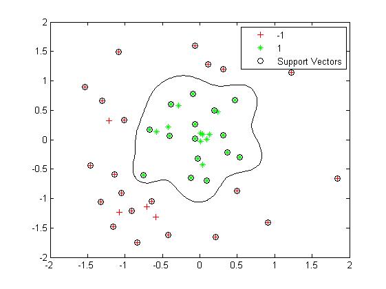
The animation you link to is doing a very different thing. It's from this article, and it shows 2d points along with a dimension representing the sum of their kernel evaluations to all other points. This is not the data mapping for a regular SVM that you're asking about, and I don't think it's useful for you to think about.

So, you're correct that there is no 3d embedding that corresponds to the classification boundary you saw. It's necessarily at least as many dimensions as the number of points you have.

The insight of the kernel trick, though, is that you don't need to actually do anything with those infinite-dimensional embeddings. You can just do the math out by evaluating $k$ between your training points, and it'll be the same as finding a hyperplane in the theoretical infinite-dimensional space.