Intuitive explanation of the bias-variance tradeoff?

Question

I am looking for an intuitive explanation of the bias-variance tradeoff, both in general and specifically in the context of linear regression.

Answer 1

Imagine some 2D data--let's say height versus weight for students at a high school--plotted on a pair of axes.

Now suppose you fit a straight line through it. This line, which of course represents a set of predicted values, has zero statistical variance. But the bias is (probably) high--i.e., it doesn't fit the data very well.

Next, suppose you model the data with a high-degree polynomial spline. You're not satisfied with the fit, so you increase the polynomial degree until the fit improves (and it will, to arbitrary precision, in fact). Now you have a situation with bias that tends to zero, but the variance is very high.

Note that the bias-variance trade-off doesn't describe a proportional relationship--i.e., if you plot bias versus variance you won't necessarily see a straight line through the origin with slope -1. In the polynomial spline example above, reducing the degree almost certainly increases the variance much less than it decreases the bias.

The bias-variance tradeoff is also embedded in the sum-of-squares error function. Below, I have rewritten (but not altered) the usual form of this equation to emphasize this:

$$ E\left(\left(y - \dot{f}(x)\right)^2\right) = \sigma^2 + \left[f(x) - \frac{1}{\kappa}\sum_{i=0}^nf(x_n)\right]^2+\frac{\sigma^2}{\kappa} $$

On the right-hand side, there are three terms: the first of these is just the irreducible error (the variance in the data itself); this is beyond our control so ignore it. The second term is the square of the bias; and the third is the variance. It's easy to see that as one goes up the other goes down--they can't both vary together in the same direction. Put another way, you can think of least-squares regression as (implicitly) finding the optimal combination of bias and variance from among candidate models.

Answer 2

Let's say you are considering catastrophic health insurance, and there is a 1% probability of getting sick which would cost 1 million dollars. The expected cost of getting sick is thus 10,000 dollars. The insurance company, wanting to make a profit, will charge you 15,000 for the policy.

Buying the policy gives an expected cost to you of 15,000, which has a variance of 0 but can be thought of as biased since it is 5,000 more than the real expected cost of getting sick.

Not buying the policy gives an expected cost of 10,000, which is unbiased since it is equal to the true expected cost of getting sick, but has a very high variance. The tradeoff here is between an approach that is consistently wrong but never by much and an approach that is correct on average but is more variable.

Answer 3

I highly recommend having a look at Caltech ML course by Yaser Abu-Mostafa, Lecture 8 (Bias-Variance Tradeoff) . Here are the outlines:

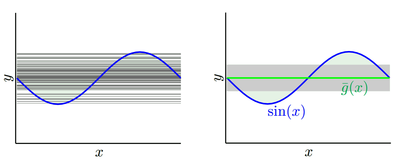
Say you are trying to learn the sine function:

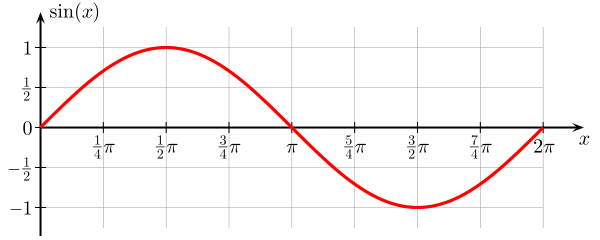
Our training set consists of only 2 data points.

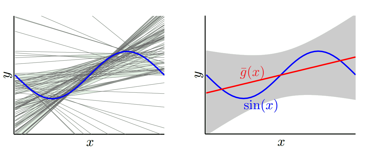
Let's try to do it with two models, $h_0(x)=b$ and $h_1(x)=ax+b$:

For $h_0(x)=b$, when we try with many different training sets (i.e. we repeatedly select 2 data points and perform the learning on them), we obtain (left graph represents all the learnt models, right graph represent their mean g and their variance (grey area)):

For $h_1(x)=ax+b$, when we try with many different training sets, we obtain:

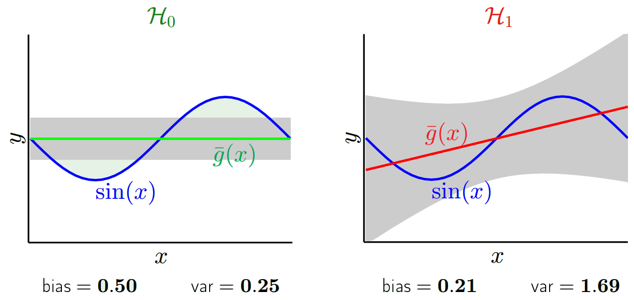
If we compare the learnt model with $h_0$ and $h_1$, we can see that $h_0$ yields more simple models than $h_1$, hence a lower variance when we consider all the models learnt with $h_0$, but the best model g (in red on the graph) learnt with $h_1$ is better than the best model learnt g with $h_0$, hence a lower bias with $h_1$:

---

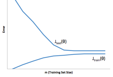
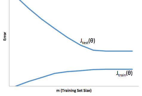
If you look at the evolution of the cost function with respect to the size of the training set (figures from Coursera - Machine Learning by Andrew Ng):

High bias:

High variance:

Answer 4

First, lets understand the meaning of bias and variance:

Suppose the center of the bulls' eye region (red) is the true mean of our target random variable that we are trying to predict. Every time we sample a set of observations and predict the value of this variable, we plot a blue dot. We have predicted correctly iff the blue dot falls inside the red region. Bias is the measure of how far off are the predicted blue dots from the center of the red region (the true mean). Intuitively, bias is a quantification of prediction error. Variance is how scattered are our predictions.

The top left is the ideal condition, but it is hard to achieve in practice, and the bottom right is the worst-case scenario, which is easy to achieve in practice. Bottom-right is usually the starting condition for randomly initialized models. Our goal is to go from the bottom-right (high-bias high-variance) situation to the top-left (low-variance low-bias).

But the problem here is: Unfortunately, achieving the lowest variance and lowest bias simultaneously is hard. (Why so? That's a deeper question). When we try to decrease one of these measures (either bias or variance), the other one increases.

Now the trade-off here is:

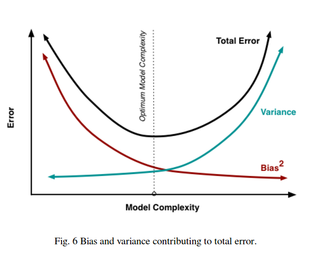
There is a sweet spot somewhere in between which produces the least prediction error in the long run.

These pictures are taken from http://scott.fortmann-roe.com/docs/BiasVariance.html . Checkout the explanations with linear regression and K-nearest neighbors for more details

Answer 5

The basic idea is that too simple a model will underfit (high bias) while too complex a model will overfit (high variance) and that bias and variance trade off as model complexity is varied.

(Neal, 2019)

However, while bias-variance tradeoff seems to hold for some simple algorithms like linear regression, or $k$-NN, it's not that simple. I'll briefly summarize some of the points made in this blog entry, by Neal (2019), and Neal et al (2018).

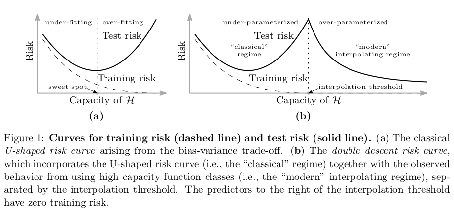
There's growing body of evidence that this is not generally true and in some machine learning algorithms we observe, so called, double descent phenomenon. There are some preliminary evidence that for random forests, gradient boosting algorithms, and neural networks this might not be the case. It was observed that wider networks (more neurons) generalize better. Moreover, as discussed by Belkin et al (2019), for overparametrized neural networks and random forests, the bias-variance curve hits certain threshold, where the model overfits, and then, as the number of parameters grows beyond the number of datapoints, the test error starts falling again with growing model complexity (see figure from the paper reproduced below).

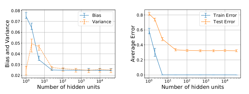
Nice example for this was given by Neal (2019), and Neal et al (2018), using simple, single layer, dense neural network, trained with stochastic gradient descent on the subset of 100 samples from MNIST. Nonetheless that the number of parameters starts exceeding the number of samples, we do not see tradeoff in terms of decrease of test set performance.

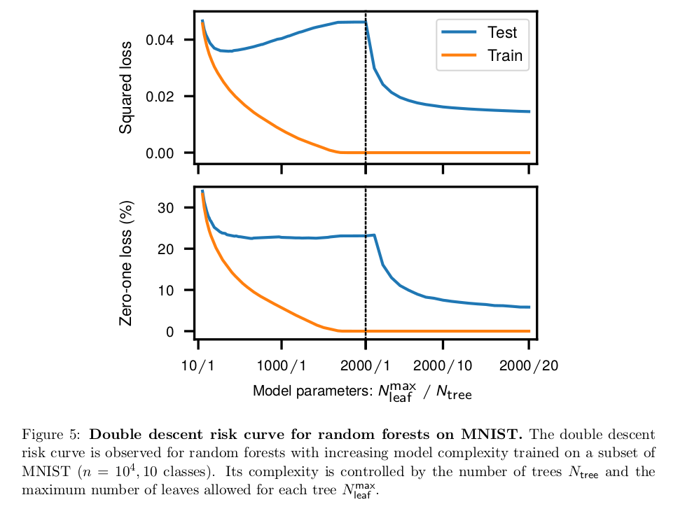
Belkin et al (2019) give even more striking example using random forest.

As discussed by Neal (2019), lack of bias-variance tradeoff for neural networks was even visible in the widely cited paper by Geman et al (1992) who did the first empirical study on this topic and popularized it. Moreover, when discussing bias-variance tradeoff, it is often shown how squared error can be decomposed into bias and variance, no matter that it does not directly apply to other error metrics, and the fact that you can decompose it does not prove anyhow that there is a tradeoff.

All this shows that we do not yet have good understanding of how and why some of the modern machine learning algorithms work, and some of our commonly held intuitions may be misleading.

---

Belkin, M., Hsub, D., Maa, S., & Mandala, S. (2019). Reconciling modern machine learning practice and the bias-variance trade-off. stat, 1050, 10.
Neal, B. (2019). On the Bias-Variance Tradeoff: Textbooks Need an Update. arXiv preprint arXiv:1912.08286.
Neal, B., Mittal, S., Baratin, A., Tantia, V., Scicluna, M., Lacoste-Julien, S., & Mitliagkas, I. (2018). A modern take on the bias-variance tradeoff in neural networks. arXiv preprint arXiv:1810.08591.

Answer 6

Here is a very simple explanation. Imagine you have a scatter plot of points {x_i,y_i} that were sampled from some distribution. You want to fit some model to it. You can choose a linear curve or a higher order polynomial curve or something else. Whatever you choose is going to be applied to predict new y values for a set of {x_i} points. Let's call these the validation set. Let's assume that you also know their true {y_i} values and we are using these just to test out model.

The predicted values are going to be different from the real values. We can measure the properties of their differences. Let's just consider a single validation point. Call it x_v and choose some model. Let's make a set of predictions for that one validation point by using say 100 different random samples for training the model. So we are going to get 100 y values. The difference between the mean of those values and the true value is called the bias. The variance of the distribution is the variance.

Depending on what model we use we can trade off between these two. Let's consider the two extremes. The lowest variance model is one where completely ignore the data. Let's say we simply predict 42 for every x. That model has zero variance across different training samples at every point. However it is clearly biased. The bias is simply 42-y_v.

One the other extreme we can choose a model which overfits as much as possible. For example fit a 100 degree polynomial to 100 data points. Or alternatively, linearly interpolate between nearest neighbors. This has low bias. Why? Because for any random sample the neighboring points to x_v will fluctuate widely but they will interpolate higher just about as often as they will interpolate low. So on average across the samples, they will cancel out and the bias will therefore be very low unless the true curve has lots of high frequency variation.

Hoever these overfit models have large variance across the random samples because they are not smoothing the data. The interpolation model just uses two data points to predict the intermediate one and these therefore create a lot of noise.

Note that the bias is measured at a single point. It doesn't matter if it is positive or negative. It is still a bias at any given x. The biases averaged over all the x values will probably be small but that doesn't make it unbiased.

One more example. Say you are trying to predict the temperature at set of locations in the US at some time. Let's assume you have 10,000 training points. Again, you can get a low variance model by doing something simple by just returning the average. But this will be biased low in the state of Florida and biased high in the state of Alaska. You'd be better if you used the average for each state. But even then, you will be biased high in the winter and low in the summer. So now you include the month in your model. But you're still going to be biased low in Death Valley and high on Mt Shasta. So now you go to the zip code level of granularity. But eventually if you keep doing this to reduce the bias, you run out of data points. Maybe for a given zip code and month, you have only one data point. Clearly this is going to create lots of variance. So you see having a more complicated model lowers the bias at the expense of variance.

So you see there is a trade off. Models that are smoother have lower variance across training samples but don't capture the real shape of the curve as well. Models that are less smooth can better capture the curve but at the expense of being noisier. Somewhere in the middle is a Goldilocks model that makes an acceptable tradeoff between the two.

Answer 7

Imagine if model building task could be repeated for different training datasets, i.e. we train a new model for different dataset every time(shown in the figure below). If we fix a test data point and evaluate model prediction on this point, the predictions will be varied due to randomness in the model generation process. From the below figure for this situation, P_1, P_2, …, P_n are different predictions and random too.

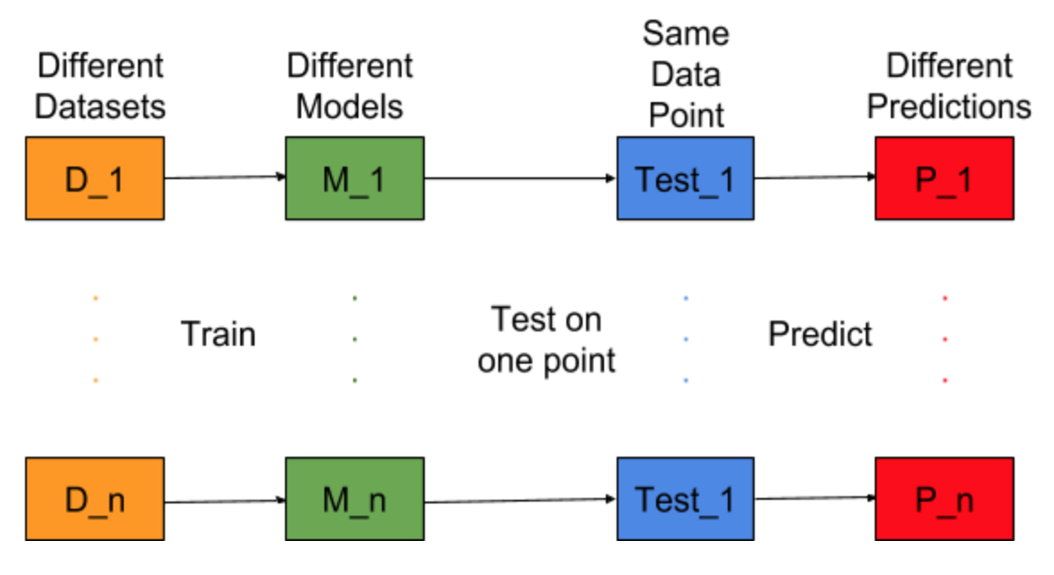
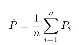
Let the mean of predictions be -

Bias Error is due to the difference between mean of these predictions and the correct value.

Variance Error is nothing but the variance in these predictions, i.e. how varied are these predictions.

This is the intuition behind bias and variance error.

For detailed explanation visit right intuition behind bias variance tradeoff