68
$\begingroup$

I learned in my linear models class that if two predictors are correlated and both are included in a model, one will be insignificant. For example, assume the size of a house and the number of bedrooms are correlated. When predicting the cost of a house using these two predictors, one of them can be dropped because they are both providing a lot of the same information. Intuitively, this makes sense, but I have a some more technical questions:

  1. How does this effect manifest itself in p-values of the regression coefficients when including only one or including both predictors in the model?
  2. How does the variance of the regression coefficients get affected by including both predictors in the model or just having one?
  3. How do I know which predictor the model will choose to be less significant?
  4. How does including only one or including both predictors change the value/variance of my forecasted cost?
$\endgroup$
2
  • 6
    $\begingroup$ Answers to some of your questions have appeared in other threads, such as at stats.stackexchange.com/a/14528, which describes a situation in which every one of a set of only mildly correlated predictors appears to be insignificant even though they collectively belong in the model. It's a good set of questions but leads to a large number of considerations and techniques; entire books have been written about them. See, for instance, Frank Harrell's Regression Modeling Strategies. $\endgroup$
    – whuber
    Commented Feb 11, 2014 at 22:39
  • 1
    $\begingroup$ Using the house size and bedrooms, you can see that insignificance is not guaranteed if correlation is different from 1 or -1. There actually exist 2-bedroom and 3-bedroom houses with the same size, and their costs may be (significantly) different, making both predictors significant. However, size in square meters and size in square feet have correlation=1 and one of them can always be dropped. $\endgroup$
    – Pere
    Commented Jan 20, 2017 at 12:51

3 Answers 3

51
$\begingroup$

The topic you are asking about is multicollinearity. You might want to read some of the threads on CV categorized under the tag. @whuber's answer linked above in particular is also worth your time.


The assertion that "if two predictors are correlated and both are included in a model, one will be insignificant", is not correct. If there is a real effect of a variable, the probability that variable will be significant is a function of several things, such as the magnitude of the effect, the magnitude of the error variance, the variance of the variable itself, the amount of data you have, and the number of other variables in the model. Whether the variables are correlated is also relevant, but it doesn't override these facts. Consider the following simple demonstration in R:

library(MASS)    # allows you to generate correlated data
set.seed(4314)   # makes this example exactly replicable

# generate sets of 2 correlated variables w/ means=0 & SDs=1
X0 = mvrnorm(n=20,   mu=c(0,0), Sigma=rbind(c(1.00, 0.70),    # r=.70
                                            c(0.70, 1.00)) )
X1 = mvrnorm(n=100,  mu=c(0,0), Sigma=rbind(c(1.00, 0.87),    # r=.87
                                            c(0.87, 1.00)) )
X2 = mvrnorm(n=1000, mu=c(0,0), Sigma=rbind(c(1.00, 0.95),    # r=.95
                                            c(0.95, 1.00)) )
y0 = 5 + 0.6*X0[,1] + 0.4*X0[,2] + rnorm(20)    # y is a function of both
y1 = 5 + 0.6*X1[,1] + 0.4*X1[,2] + rnorm(100)   #  but is more strongly
y2 = 5 + 0.6*X2[,1] + 0.4*X2[,2] + rnorm(1000)  #  related to the 1st

# results of fitted models (skipping a lot of output, including the intercepts)
summary(lm(y0~X0[,1]+X0[,2]))
#             Estimate Std. Error t value Pr(>|t|)    
# X0[, 1]       0.6614     0.3612   1.831   0.0847 .     # neither variable
# X0[, 2]       0.4215     0.3217   1.310   0.2075       #  is significant
summary(lm(y1~X1[,1]+X1[,2]))
#             Estimate Std. Error t value Pr(>|t|)    
# X1[, 1]      0.57987    0.21074   2.752  0.00708 **    # only 1 variable
# X1[, 2]      0.25081    0.19806   1.266  0.20841       #  is significant
summary(lm(y2~X2[,1]+X2[,2]))
#             Estimate Std. Error t value Pr(>|t|)    
# X2[, 1]      0.60783    0.09841   6.177 9.52e-10 ***   # both variables
# X2[, 2]      0.39632    0.09781   4.052 5.47e-05 ***   #  are significant

The correlation between the two variables is lowest in the first example and highest in the third, yet neither variable is significant in the first example and both are in the last example. The magnitude of the effects is identical in all three cases, and the variances of the variables and the errors should be similar (they are stochastic, but drawn from populations with the same variance). The pattern we see here is due primarily to my manipulating the $N$s for each case.


The key concept to understand to resolve your questions is the variance inflation factor (VIF). The VIF is how much the variance of your regression coefficient is larger than it would otherwise have been if the variable had been completely uncorrelated with all the other variables in the model. Note that the VIF is a multiplicative factor, if the variable in question is uncorrelated the VIF=1. A simple understanding of the VIF is as follows: you could fit a model predicting a variable (say, $X_1$) from all other variables in your model (say, $X_2$), and get a multiple $R^2$. The VIF for $X_1$ would be $1/(1-R^2)$. Let's say the VIF for $X_1$ were $10$ (often considered a threshold for excessive multicollinearity), then the variance of the sampling distribution of the regression coefficient for $X_1$ would be $10\times$ larger than it would have been if $X_1$ had been completely uncorrelated with all the other variables in the model.

Thinking about what would happen if you included both correlated variables vs. only one is similar, but slightly more complicated than the approach discussed above. This is because not including a variable means the model uses less degrees of freedom, which changes the residual variance and everything computed from that (including the variance of the regression coefficients). In addition, if the non-included variable really is associated with the response, the variance in the response due to that variable will be included into the residual variance, making it larger than it otherwise would be. Thus, several things change simultaneously (the variable is correlated or not with another variable, and the residual variance), and the precise effect of dropping / including the other variable will depend on how those trade off. The best way to think through this issue is based on the counterfactual of how the model would differ if the variables were uncorrelated instead of correlated, rather than including or excluding one of the variables.


Armed with an understanding of the VIF, here are the answers to your questions:

  1. Because the variance of the sampling distribution of the regression coefficient would be larger (by a factor of the VIF) if it were correlated with other variables in the model, the p-values would be higher (i.e., less significant) than they otherwise would.
  2. The variances of the regression coefficients would be larger, as already discussed.
  3. In general, this is hard to know without solving for the model. Typically, if only one of two is significant, it will be the one that had the stronger bivariate correlation with $Y$.
  4. How the predicted values and their variance would change is quite complicated. It depends on how strongly correlated the variables are and the manner in which they appear to be associated with your response variable in your data. Regarding this issue, it may help you to read my answer here: Is there a difference between 'controlling for' and 'ignoring' other variables in multiple regression?
$\endgroup$
5
$\begingroup$

As @whuber noted, this is a complex question. However, the first sentence of your post is a vast simplification. It is often the case that two (or more) variables will be correlated and both related to the dependent variable. Whether they are significant or not depends on both effect size and cell size.

In your example, suppose that, for a given size of house, people preferred fewer rooms (at least in NYC, this isn't unreasonable - it would indicate older buildings, more solid walls etc, and might be a marker for neighborhood). Then both could be significant, in opposite directions!

Or, suppose the two variables were house size and neighborhood - these would be correlated, surely, larger houses in better neighborhoods - but they could still both be significant and would surely both be related to house price.

Also, using only "correlated" masks complexities. Variables can be strongly related without being correlated.

$\endgroup$
5
$\begingroup$

This is more of comment, but I wanted to include a graph and some code.

I think the statement "if two predictors are correlated and both are included in a model, one will be insignificant" is false if you mean "only one." Binary statistical significance cannot be used for variable selection.

Here's my counterexample using a regression of body fat percentage on thigh circumference, skin fold thickness*, and mid arm circumference:

. webuse bodyfat, clear
(Body Fat)

. reg bodyfat thigh triceps midarm

      Source |       SS       df       MS              Number of obs =      20
-------------+------------------------------           F(  3,    16) =   21.52
       Model |  396.984607     3  132.328202           Prob > F      =  0.0000
    Residual |  98.4049068    16  6.15030667           R-squared     =  0.8014
-------------+------------------------------           Adj R-squared =  0.7641
       Total |  495.389513    19  26.0731323           Root MSE      =    2.48

------------------------------------------------------------------------------
     bodyfat |      Coef.   Std. Err.      t    P>|t|     [95% Conf. Interval]
-------------+----------------------------------------------------------------
       thigh |  -2.856842   2.582015    -1.11   0.285    -8.330468    2.616785
     triceps |   4.334085   3.015511     1.44   0.170    -2.058512    10.72668
      midarm |  -2.186056   1.595499    -1.37   0.190    -5.568362     1.19625
       _cons |   117.0844   99.78238     1.17   0.258    -94.44474    328.6136
------------------------------------------------------------------------------

. corr bodyfat thigh triceps midarm 
(obs=20)

             |  bodyfat    thigh  triceps   midarm
-------------+------------------------------------
     bodyfat |   1.0000
       thigh |   0.8781   1.0000
     triceps |   0.8433   0.9238   1.0000
      midarm |   0.1424   0.0847   0.4578   1.0000


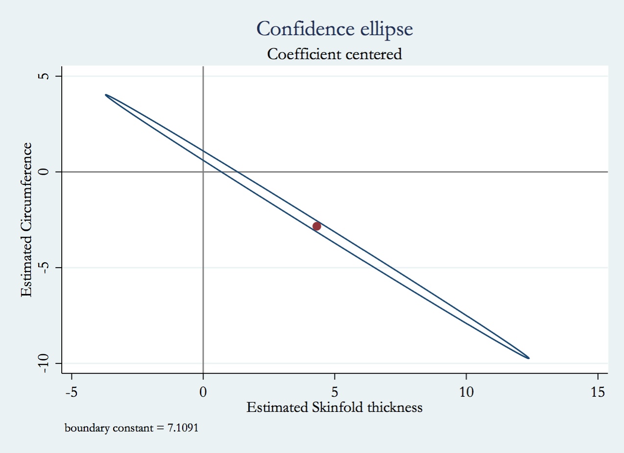
. ellip thigh triceps, coefs plot( (scatteri `=_b[thigh]' `=_b[triceps]'), yline(0, lcolor(gray)) xline(0, lcolor(gray)) legend(off))

enter image description here

As you can see from the regression table, everything is insignificant, though the p-values do vary a bit.

The last Stata command graphs the confidence region for 2 of the regression coefficients (a two dimensional analog of the familiar confidence intervals) along with the point estimates (red dot). The confidence ellipse for the skin fold thickness and thigh circumference coefficients is long, narrow and tilted, reflecting the collinearity in the regressors. There's high negative covariance between the estimated coefficients. The ellipse covers parts of the vertical and the horizontal axes, which means that we cannot reject the individual hypotheses that the $\beta$s are zero, though we can reject the joint null that both are since the ellipse does not cover the origin. In other words, either thigh and triceps are relevant for body fat, but you can't determine which one is the culprit.

So how do we know which predictors would be less significant? The variation in a regressor can be classified into two types:

  1. Variation unique to each regressor
  2. Variation that is shared by the regressors

In estimating the coefficients of each regressor, only the first will be used. Common variation is ignored since it cannot be allocated, though it is used in prediction and calculating $R^2$. When there is little unique information, the confidence will be low and coefficient variances will be high. The higher the multicollinearity, the smaller the unique variation, and the greater the variances.


*The skin fold is the width of a fold of skin taken over the triceps muscle, and measured using a caliper.

$\endgroup$
3
  • $\begingroup$ I like your example, but strictly speaking it would be a counterexample if the statement in the original question said "if [...], only one will be insignificant", but it does not have the word "only". $\endgroup$
    – amoeba
    Commented Feb 12, 2014 at 0:37
  • $\begingroup$ @amoeba That's an excellent point. I will amend my comment. $\endgroup$
    – dimitriy
    Commented Feb 12, 2014 at 0:46
  • $\begingroup$ Can you provide some formula to further illustrate: "In estimating the coefficients of each regressor, only the first will be used. Common variation is ignored since it cannot be allocated" $\endgroup$
    – mac
    Commented Jun 8, 2017 at 20:28

Your Answer

By clicking “Post Your Answer”, you agree to our terms of service and acknowledge you have read our privacy policy.

Not the answer you're looking for? Browse other questions tagged or ask your own question.