Computing the decision boundary of a linear SVM model

Question

Given the support vectors of a linear SVM, how can I compute the equation of the decision boundary?

Answer 1

The Elements of Statistical Learning, from Hastie et al., has a complete chapter on support vector classifiers and SVMs (in your case, start page 418 on the 2nd edition). Another good tutorial is Support Vector Machines in R, by David Meyer.

Unless I misunderstood your question, the decision boundary (or hyperplane) is defined by $x^T\beta + \beta_0=0$ (with $\|\beta\|=1$, and $\beta_0$ the intercept term), or as @ebony said a linear combination of the support vectors. The margin is then $2/\|\beta\|$, following Hastie et al. notations.

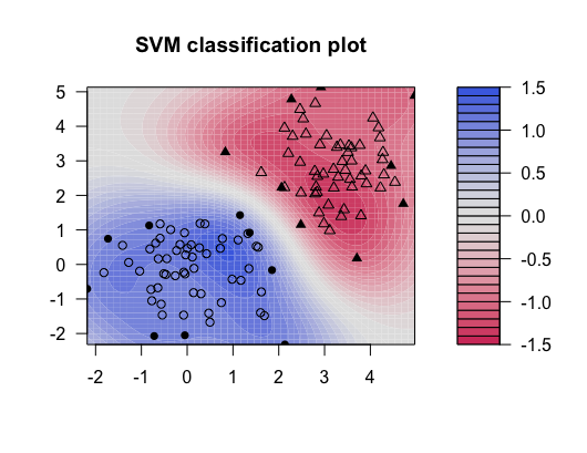
From the on-line help of ksvm() in the kernlab R package, but see also kernlab – An S4 Package for Kernel Methods in R, here is a toy example:

set.seed(101)
x <- rbind(matrix(rnorm(120),,2),matrix(rnorm(120,mean=3),,2))
y <- matrix(c(rep(1,60),rep(-1,60)))
svp <- ksvm(x,y,type="C-svc")
plot(svp,data=x)

Note that for the sake of clarity, we don't consider train and test samples. Results are shown below, where color shading helps visualizing the fitted decision values; values around 0 are on the decision boundary.

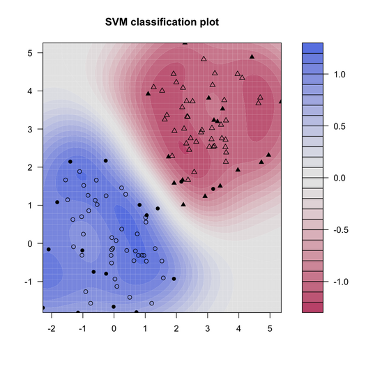
Calling attributes(svp) gives you attributes that you can access, e.g.

alpha(svp)  # support vectors whose indices may be 
            # found with alphaindex(svp)
b(svp)      # (negative) intercept 

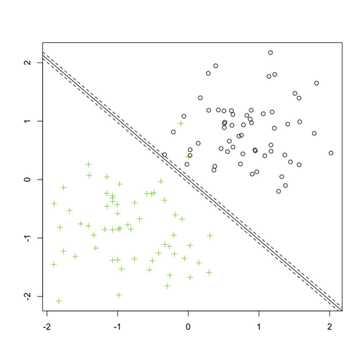
So, to display the decision boundary, with its corresponding margin, let's try the following (in the rescaled space), which is largely inspired from a tutorial on SVM made some time ago by Jean-Philippe Vert:

plot(scale(x), col=y+2, pch=y+2, xlab="", ylab="")
w <- colSums(coef(svp)[[1]] * x[unlist(alphaindex(svp)),])
b <- b(svp)
abline(b/w[1],-w[2]/w[1])
abline((b+1)/w[1],-w[2]/w[1],lty=2)
abline((b-1)/w[1],-w[2]/w[1],lty=2)

And here it is:

Answer 2

It's a linear combination of the support vectors where the coefficients are given by the Lagrange multipliers corresponding to these support vectors.

Answer 3

I was unable to verify the accepted answer above as the plots generated by the code are different from those shown in the answer.

library(kernlab)
set.seed(101)
x <- rbind(matrix(rnorm(120),,2),matrix(rnorm(120,mean=3),,2))
y <- matrix(c(rep(1,60),rep(-1,60)))
# it is important that your outcome is coded as c(-1, 1), 
# the intercept calculation will be incorrect if your outcome 
# is coded as something else (for example, c(1,2)).
svp <- ksvm(x,y,type="C-svc")
plot(svp,data=x)

w <- colSums(coef(svp)[[1]] * x[unlist(alphaindex(svp)),])
> w
[1] -16.79469 -14.39577

b <- b(svp)
> b
[1] 0.04062546

icpt = b/w[1]
slp = -w[2]/w[1]
> slp
[1] -0.8571617
> icpt
[1] -0.002418946

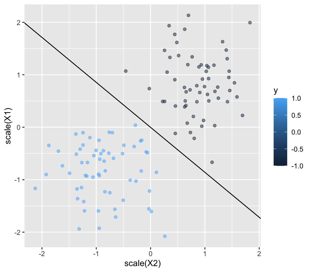
dat = data.frame(x,y)
ggplot(dat, aes(x=scale(X2), y=scale(X1), color=y)) +
  geom_point(alpha=.5) +
  geom_abline(slope = slp, intercept = icpt)

Unfortunately, this does not appear to be the optimal linear decision boundary... just from a visual examination it does not appear to be the maximum margin classifier/regression.

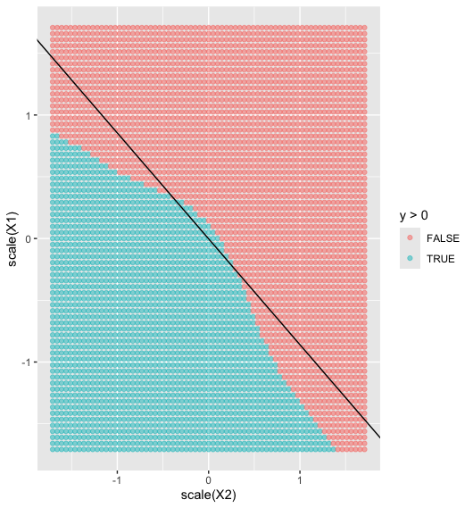
dfchk = expand.grid(X1 = seq(-2,5,.1), X2 = seq(-2,5,.1)) %>%
  mutate(y = predict(svp, .))
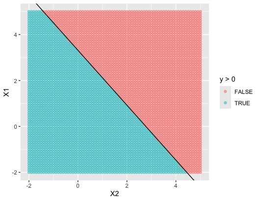
ggplot(dfchk, aes(x=scale(X2), y=scale(X1), color=y>0)) +
  geom_point(alpha=.5) +
  geom_abline(slope = slp, intercept = icpt)

Indeed, checking on a dense grid shows that this is not the correct decision boundary - it doesn't appear to be a linear SVM at all, so perhaps that is the issue.

tidymodels

I wanted to verify with another package, so here's what I found with tidymodels:

library(tidymodels)
library(LiblineaR)
svm_model <- svm_linear(mode = "regression")
svm_recipe <- recipe(y ~ X1 + X2, data = dat)
svm_flow <- workflow() %>%
  add_model(svm_model) %>%
  add_recipe(svm_recipe)
svm_fit <- svm_flow %>%
  fit(data = dat)

coeffs = svm_fit %>%
  extract_fit_parsnip() %>%
  tidy() %>% 
  pull(estimate)

> coeffs
       X1        X2      Bias 
-0.251783 -0.301117  0.834984 

slp = -coeffs[["X2"]]/coeffs[["X1"]]
icpt = -coeffs[["Bias"]]/coeffs[["X1"]]
> slp
[1] -1.19594
> icpt
[1] 3.31628

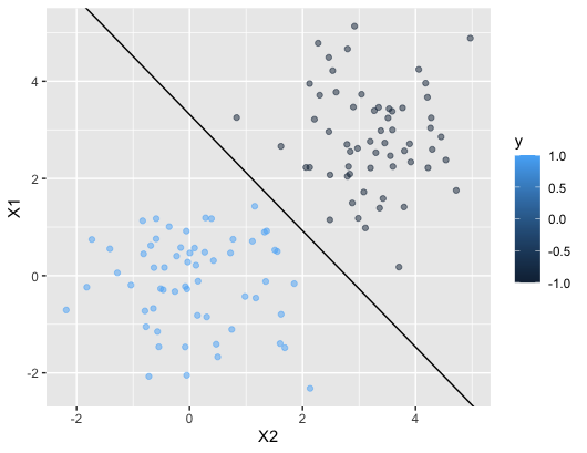
ggplot(dat, aes(x=X2, y=X1, color=y)) +
  geom_point(alpha=.5) +
  geom_abline(slope = slp, intercept = icpt)

Visually, this looks better but we can check our work:

# check on a dense grid:
dfchk = expand.grid(X1 = seq(-2,5,.1), X2 = seq(-2,5,.1)) %>%
  mutate(y = predict(svm_fit, .) %>% pull(.pred))
ggplot(dfchk, aes(x=X2, y=X1, color=y>0)) +
  geom_point(alpha=.5) +
  geom_abline(slope = slp, intercept = icpt)

Looks good to me.