Suppression effect in regression: definition and visual explanation/depiction

Question

What is a suppressor variable in multiple regression and what might be the ways to display suppression effect visually (its mechanics or its evidence in results)? I'd like to invite everybody who has a thought, to share.

Answer 1

There exist a number of frequenly mentioned regressional effects which conceptually are different but share much in common when seen purely statistically (see e.g. this paper "Equivalence of the Mediation, Confounding and Suppression Effect" by David MacKinnon et al., or Wikipedia articles):

• Mediator: IV which conveys effect (totally of partly) of another IV to the DV.
• Confounder: IV which constitutes or precludes, totally or partly, effect of another IV to the DV.
• Moderator: IV which, varying, manages the strength of the effect of another IV on the DV. Statistically, it is known as interaction between the two IVs.
• Suppressor: IV (a mediator or a moderator conceptually) which inclusion strengthens the effect of another IV on the DV.

I'm not going to discuss to what extent some or all of them are technically similar (for that, read the paper linked above). My aim is to try to show graphically what suppressor is. The above definition that "suppressor is a variable which inclusion strengthens the effect of another IV on the DV" seems to me potentially broad because it does not tell anything about mechanisms of such enhancement. Below I'm discussing one mechanism - the only one I consider to be suppression. If there are other mechanisms as well (as for right now, I haven't tried to meditate of any such other) then either the above "broad" definition should be considered imprecise or my definition of suppression should be considered too narrow.

Definition (in my understanding)

Suppressor is the independent variable which, when added to the model, raises observed R-square mostly due to its accounting for the residuals left by the model without it, and not due to its own association with the DV (which is comparatively weak). We know that the increase in R-square in response to adding a IV is the squared part correlation of that IV in that new model. This way, if the part correlation of the IV with the DV is greater (by absolute value) than the zero-order $r$ between them, that IV is a suppressor.

So, a suppressor mostly "suppresses" the error of the reduced model, being weak as a predictor itself. The error term is the complement to the prediction. The prediction is "projected on" or "shared between" the IVs (regression coefficients), and so is the error term ("complements" to the coefficients). The suppressor suppresses such error components unevenly: greater for some IVs, lesser for other IVs. For those IVs "whose" such components it suppresses greatly it lends considerable facilitating aid by actually raising their regression coefficients.

Not strong suppressing effects occurs often and wildly (an example on this site). Strong suppression is typically introduced consciously. A researcher seeks for a characteristic which must correlate with the DV as weak as possible and at the same time would correlate with something in the IV of interest which is considered irrelevant, prediction-void, in respect to the DV. He enters it to the model and gets considerable increase in that IV's predictive power. The suppressor's coefficient is typically not interpreted.

I could summarize my definition as follows [up on @Jake's answer and @gung's comments]:

• Formal (statistical) definition: suppressor is IV with part correlation larger than zero-order correlation (with the dependent).
• Conceptual (practical) definition: the above formal definition + the zero-order correlation is small, so that the suppressor is not a sound predictor itself.

"Suppessor" is a role of a IV in a specific model only, not the characteristic of the separate variable. When other IVs are added or removed, the suppressor can suddenly stop suppressing or resume suppressing or change the focus of its suppressing activity.

Normal regression situation

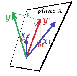
The first picture below shows a typical regression with two predictors (we'll speak of linear regression). The picture is copied from here where it is explained in more details. In short, moderately correlated (= having acute angle between them) predictors $X_1$ and $X_2$ span 2-dimesional space "plane X". The dependent variable $Y$ is projected onto it orthogonally, leaving the predicted variable $Y'$ and the residuals with st. deviation equal to the length of $e$. R-square of the regression is the angle between $Y$ and $Y'$, and the two regression coefficients are directly related to the skew coordinates $b_1$ and $b_2$, respectively. This situation I've called normal or typical because both $X_1$ and $X_2$ correlate with $Y$ (oblique angle exists between each of the independents and the dependent) and the predictors compete for the prediction because they are correlated.

Suppression situation

It is shown on the next picture. This one is like the previous; however $Y$ vector now directs somewhat away from the viewer and $X_2$ changed its direction considerably. $X_2$ acts as a suppressor. Note first of all that it hardly correlates with $Y$. Hence it cannot be a valuable predictor itself. Second. Imagine $X_2$ is absent and you predict only by $X_1$; the prediction of this one-variable regression is depicted as $Y^*$ red vector, the error as $e^*$ vector, and the coefficient is given by $b^*$ coordinate (which is the endpoint of $Y^*$).

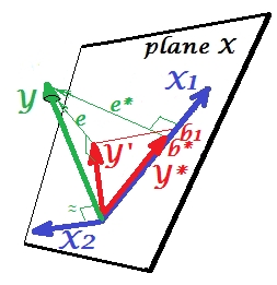
Now bring yourself back to the full model and notice that $X_2$ is fairly correlated with $e^*$. Thus, $X_2$ when introduced in the model, can explain a considerable portion of that error of the reduced model, cutting down $e^*$ to $e$. This constellation: (1) $X_2$ is not a rival to $X_1$ as a predictor; and (2) $X_2$ is a dustman to pick up unpredictedness left by $X_1$, - makes $X_2$ a suppressor. As a result of its effect, predictive strength of $X_1$ has grown to some extent: $b_1$ is larger than $b^*$.

Well, why is $X_2$ called a suppressor to $X_1$ and how can it reinforce it when "suppressing" it? Look at the next picture.

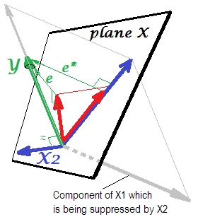
It is exactly the same as the previous. Think again of the model with the single predictor $X_1$. This predictor could of course be decomposed in two parts or components (shown in grey): the part which is "responsible" for prediction of $Y$ (and thus coinciding with that vector) and the part which is "responsible" for the unpredictedness (and thus parallel to $e^*$). It is this second part of $X_1$ - the part irrelevant to $Y$ - is suppressed by $X_2$ when that suppressor is added to the model. The irrelevant part is suppressed and thus, given that the suppressor doesn't itself predict $Y$ any much, the relevant part looks stronger. A suppressor is not a predictor but rather a facilitator for another/other predictor/s. Because it competes with what impedes them to predict.

Sign of the suppressor's regression coefficient

It is the sign of the correlation between the suppressor and the error variable $e^*$ left by the reduced (without-the-suppressor) model. In the depiction above, it is positive. In other settings (for example, revert the direction of $X_2$) it could be negative.

Suppression example

Example data:

         y         x1         x2

1.64454000  .35118800 1.06384500
1.78520400  .20000000 -1.2031500
-1.3635700 -.96106900 -.46651400
 .31454900  .80000000 1.17505400
 .31795500  .85859700 -.10061200
 .97009700 1.00000000 1.43890400
 .66438800  .29267000 1.20404800
-.87025200 -1.8901800 -.99385700
1.96219200 -.27535200 -.58754000
1.03638100 -.24644800 -.11083400
 .00741500 1.44742200 -.06923400
1.63435300  .46709500  .96537000
 .21981300  .34809500  .55326800
-.28577400  .16670800  .35862100
1.49875800 -1.1375700 -2.8797100
1.67153800  .39603400 -.81070800
1.46203600 1.40152200 -.05767700
-.56326600 -.74452200  .90471600
 .29787400 -.92970900  .56189800
-1.5489800 -.83829500 -1.2610800

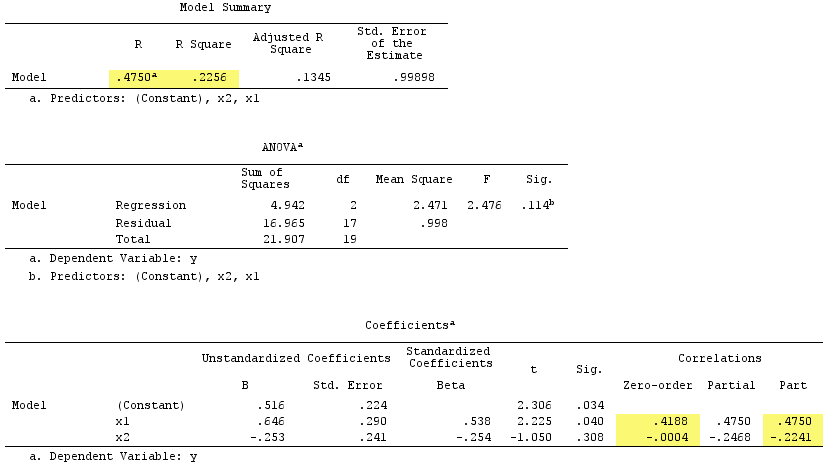
Linear regression results:

Observe that $X_2$ served as suppressor. Its zero-order correlation with $Y$ is practically zero but its part correlation is much larger by magnitude, $-.224$. It strengthened to some extent the predictive force of $X_1$ (from r $.419$, a would-be beta in simple regression with it, to beta $.538$ in the multiple regression).

According to the formal definition, $X_1$ appeared a suppressor too, because its part correlation is greater than its zero-order correlation. But that is because we have only two IV in the simple example. Conceptually, $X_1$ isn't a suppressor because its $r$ with $Y$ is not about $0$.

By way, sum of squared part correlations exceeded R-square: .4750^2+(-.2241)^2 = .2758 > .2256, which would not occur in normal regressional situation (see the Venn diagram below).

Suppression and coefficient's sign change

Adding a variable that will serve a supressor may as well as may not change the sign of some other variables' coefficients. "Suppression" and "change sign" effects are not the same thing. Moreover, I believe that a suppressor can never change sign of those predictors whom they serve suppressor. (It would be a shocking discovery to add the suppressor on purpose to facilitate a variable and then to find it having become indeed stronger but in the opposite direction! I'd be thankful if somebody could show me it is possible.)

Suppression and coefficient strengthening

To cite an earlier passage: "For those IVs "whose" such components [error components] it suppresses greatly the suppressor lends considerable facilitating aid by actually raising their regression coefficients". Indeed, in our Example above, $X_2$, the suppressor, raised the coefficient for $X_1$. Such enhancement of the unique predictive power of another regressor is often the aim of a suppressor to a model but it is not the definition of suppressor or of suppression effect. For, the aforementioned enhancement of another predictor's capacity via adding more regressors can easily occure in a normal regressional situation without those regressors being suppressors. Here is an example.

   y       x1       x2       x3

   1        1        1        1
   3        2        2        6
   2        3        3        5
   3        2        4        2
   4        3        5        9
   3        4        4        2
   2        5        3        3
   3        6        4        4
   4        7        5        5
   5        6        6        6
   4        5        7        5
   3        4        5        5
   4        5        3        5
   5        6        4        6
   6        7        5        4
   5        8        6        6
   4        2        7        7
   5        3        8        8
   6        4        9        4
   5        5        3        3
   4        6        4        2
   3        2        1        1
   4        3        5        4
   5        4        6        5
   6        9        5        4
   5        8        3        3
   3        5        5        2
   2        6        6        1
   3        7        7        5
   5        8        8        8

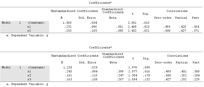
Regressions results without and with $X_3$:

Inclusion of $X_3$ in the model raised the beta of $X_1$ from $.381$ to $.399$ (and its corresponding partial correlation with $Y$ from $.420$ to $.451$). Still, we find no suppressor in the model. $X_3$'s part correlation ($.229$) is not greater than its zero-order correlation ($.427$). Same is for the other regressors. "Facilitation" effect was there, but not due to "suppression" effect. Definition of a suppessor is different from just strenghtening/facilitation; and it is about picking up mostly errors, due to which the part correlation exceeds the zero-order one.

Suppression and Venn diagram

Normal regressional situation is often explained with the help of Venn diagram.

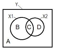
A+B+C+D = 1, all $Y$ variability. B+C+D area is the variability accounted by the two IV ($X_1$ and $X_2$), the R-square; the remaining area A is the error variability. B+C = $r_{YX_1}^2$; D+C = $r_{YX_2}^2$, Pearson zero-order correlations. B and D are the squared part (semipartial) correlations: B = $r_{Y(X_1.X_2)}^2$; D = $r_{Y(X_2.X_1)}^2$. B/(A+B) = $r_{YX_1.X_2}^2$ and D/(A+D) = $r_{YX_2.X_1}^2$ are the squared partial correlations which have the same basic meaning as the standardized regression coefficients betas.

According to the above definition (which I stick to) that a suppressor is the IV with part correlation greater than zero-order correlation, $X_2$ is the suppressor if D area > D+C area. That cannot be displayed on Venn diagram. (It would imply that C from the view of $X_2$ is not "here" and is not the same entity than C from the view of $X_1$. One must invent perhaps something like multilayered Venn diagram to wriggle oneself to show it.)

---

P.S. Upon finishing my answer I found this answer (by @gung) with a nice simple (schematic) diagram, which seems to be in agreement with what I showed above by vectors.

Answer 2

Here is another geometric view of suppression, but rather than being in the observation space as @ttnphns's example is, this one is in the variable space, the space where everyday scatterplots live.

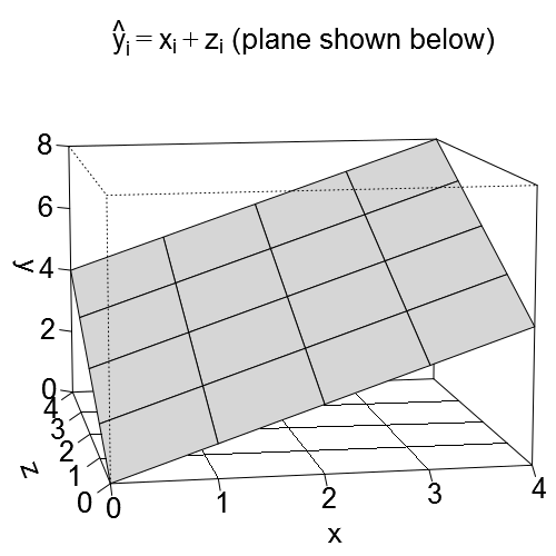
Consider a regression $\hat{y}_i=x_i+z_i$, that is, the intercept is 0 and both predictors have a partial slope of 1. Now, the predictors $x$ and $z$ may themselves be correlated. We will consider two cases: first the case where $x$ and $z$ are positively correlated, which I will call the "confounding" case (characterized by the secondary regression $\hat{x}_i=\frac{1}{2}z_i$), and second the case where $x$ and $z$ are negatively correlated, which I will call the "suppression" case (with secondary regression $\hat{x}_i=-\frac{1}{2}z_i$).

We can plot our regression equation as a plane in the variable space that looks like this:

Confounding case

Let's consider the slope for the $x$ predictor in the confounding case. To say that the other predictor $z$ is serving as a confounding variable is to say that when we look at a simple regression of $y$ on $x$, the effect of $x$ here is stronger than is the effect of x in a multiple regression of $y$ on $x$ and $z$, where we partial out the effect of $z$. The effect of $x$ that we observe in the simple regression is, in some sense (not necessarily causal), partially due to the effect of $z$, which is positively associated with both $y$ and $x$, but not included in the regression. (For the purposes of this answer I will use "the effect of $x$" to refer to the slope of $x$.)

We will call the slope of $x$ in the simple linear regression the "simple slope" of $x$ and the slope of $x$ in the multiple regression the "partial slope" of $x$. Here is what the simple and partial slopes of $x$ look like as vectors on the regression plane:

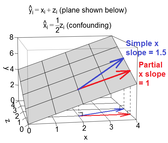
The partial slope of x is perhaps easier to understand. It is shown in red above. It is the slope of a vector that moves along the plane in such a way that $x$ is increasing, but $z$ is held constant. This is what it means to "control for" $z$.

The simple slope of $x$ is slightly more complicated because it implicitly also includes part of the effect of the $z$ predictor. It is shown in blue above. The simple slope of $x$ is the slope of a vector that moves along the plane in such a way that $x$ is increasing, and $z$ also is increasing (or decreasing) to whatever extent $x$ and $z$ are associated in the dataset. In the confounding case, we set things up so that the relationship between $x$ and $z$ was such that when we move up one unit on $x$, we also move up half a unit on $z$ (this comes from the secondary regression $\hat{x}_i=\frac{1}{2}z_i$). And since one-unit changes in both $x$ and $z$ are separately associated with one-unit changes in $y$, this means that the simple slope of $x$ in this case will be $\Delta x + \Delta z = 1 + \frac{1}{2} = 1.5$.

So when we control for $z$ in the multiple regression, the effect of $x$ appears to be smaller than it was in the simple regression. We can see this visually above in the fact that the red vector (representing the partial slope) is less steep than the blue vector (representing the simple slope). The blue vector is really the result of adding two vectors, the red vector and another vector (not shown) representing the half the partial slope of $z$.

Okay, now we turn to the slope for the $x$ predictor in the suppression case. If you followed all of the above, this is a really easy extension.

Suppression case

To say that the other predictor $z$ is serving as a supressor variable is to say that when we look at a simple regression of $y$ on $x$, the effect of $x$ here is weaker than is the effect of x in a multiple regression of $y$ on $x$ and $z$, where we partial out the effect of $z$. (Note that in extreme cases, the effect of $x$ in the multiple regression might even flip directions! But I am not considering that extreme case here.) The intution behind the terminology is that it appears that in the simple regression case, the effect of $x$ was being "suppressed" by the omitted $z$ variable. And when we include $z$ in the regression, the effect of $x$ emerges clearly for us to see, where we couldn't see it as clearly before. Here is what the simple and partial slopes of $x$ look like as vectors on the regression plane in the suppression case:

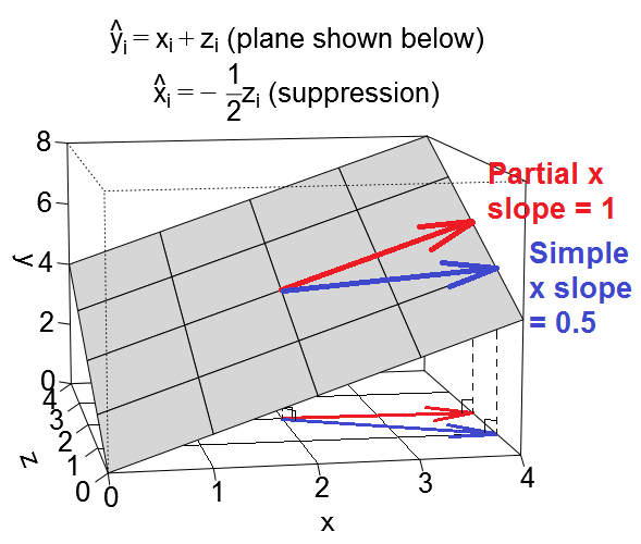
So when we control for $z$ in the multiple regression, the effect of $x$ appears to increase relative to what it was in the simple regression. We can see this visually above in the fact that the red vector (representing the partial slope) is steeper than the blue vector (representing the simple slope). In this case the secondary regression was $\hat{x}_i=-\frac{1}{2}z_i$, so a one-unit increase in $x$ is associated with a half-unit decrease in $z$, which in turn leads to a half-unit decrease in $y$. So ultimately the simple slope of $x$ in this case will be $\Delta x + \Delta z = 1 + -\frac{1}{2} = 0.5$. As before, the blue vector is really the result of adding two vectors, the red vector and another vector (not shown) representing half of the reverse of the partial slope of $z$.

Illustrative datasets

In case you want to play around with these examples, here is some R code for generating data conforming to the example values and running the various regressions.

library(MASS) # for mvrnorm()
set.seed(7310383)

# confounding case --------------------------------------------------------

mat <- rbind(c(5,1.5,1.5),
             c(1.5,1,.5),
             c(1.5,.5,1))
dat <- data.frame(mvrnorm(n=50, mu=numeric(3), empirical=T, Sigma=mat))
names(dat) <- c("y","x","z")

cor(dat)
#           y         x         z
# y 1.0000000 0.6708204 0.6708204
# x 0.6708204 1.0000000 0.5000000
# z 0.6708204 0.5000000 1.0000000

lm(y ~ x, data=dat)
# 
# Call:
#   lm(formula = y ~ x, data = dat)
# 
# Coefficients:
#   (Intercept)            x  
#     -1.57e-17     1.50e+00  

lm(y ~ x + z, data=dat)
# 
# Call:
#   lm(formula = y ~ x + z, data = dat)
# 
# Coefficients:
#   (Intercept)            x            z  
#      3.14e-17     1.00e+00     1.00e+00  
# @ttnphns comment: for x, zero-order r = .671 > part r = .387
#                   for z, zero-order r = .671 > part r = .387

lm(x ~ z, data=dat)
# 
# Call:
#   lm(formula = x ~ z, data = dat)
# 
# Coefficients:
#   (Intercept)            z  
#     6.973e-33    5.000e-01 

# suppression case --------------------------------------------------------

mat <- rbind(c(2,.5,.5),
             c(.5,1,-.5),
             c(.5,-.5,1))
dat <- data.frame(mvrnorm(n=50, mu=numeric(3), empirical=T, Sigma=mat))
names(dat) <- c("y","x","z")

cor(dat)
#           y          x          z
# y 1.0000000  0.3535534  0.3535534
# x 0.3535534  1.0000000 -0.5000000
# z 0.3535534 -0.5000000  1.0000000

lm(y ~ x, data=dat)
# 
# Call:
#   lm(formula = y ~ x, data = dat)
# 
# Coefficients:
#   (Intercept)            x  
#    -4.318e-17    5.000e-01  

lm(y ~ x + z, data=dat)
# 
# Call:
#   lm(formula = y ~ x + z, data = dat)
# 
# Coefficients:
#   (Intercept)            x            z  
#    -3.925e-17    1.000e+00    1.000e+00  
# @ttnphns comment: for x, zero-order r = .354 < part r = .612
#                   for z, zero-order r = .354 < part r = .612

lm(x ~ z, data=dat)
# 
# Call:
#   lm(formula = x ~ z, data = dat)
# 
# Coefficients:
#   (Intercept)            z  
#      1.57e-17    -5.00e-01  

Answer 3

Here is how I think about the suppressor effect. But please let me know if I am wrong.

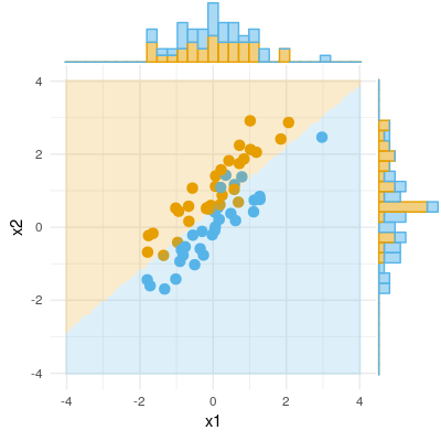
Here is an example of a binary outcome (classification, logistic regression). We can see that there is no significant difference in X1, there is no difference in X2, but put X1 and X2 together (i.e. correct x1 for x2 or vice versa) and samples can be classified almost perfectly and thus the variables are now highly significant.