13
$\begingroup$

I'm trying to test various functional data analysis approaches. Ideally, i'd like to test the panel of approaches i have on simulated functional data. I've tried to generate simulated FD using an approach based on a summing Gaussian noises (code below), but the resulting curves look much too rugged compared to the real thing.

I was wondering whether somebody had a pointer to functions/ideas to generate more realistic looking simulated functional data. In particular, these should be smooth. I'm completely new to this field so any advice is welcomed.

library("MASS")
library("caTools")
VCM<-function(cont,theta=0.99){
    Sigma<-matrix(rep(0,length(cont)^2),nrow=length(cont))
    for(i in 1:nrow(Sigma)){
        for (j in 1:ncol(Sigma)) Sigma[i,j]<-theta^(abs(cont[i]-cont[j]))
    }
    return(Sigma)
}


t1<-1:120
CVC<-runmean(cumsum(rnorm(length(t1))),k=10)
VMC<-VCM(cont=t1,theta=0.99)
sig<-runif(ncol(VMC))
VMC<-diag(sig)%*%VMC%*%diag(sig)
DTA<-mvrnorm(100,rep(0,ncol(VMC)),VMC)  

DTA<-sweep(DTA,2,CVC)
DTA<-apply(DTA,2,runmean,k=5)
matplot(t(DTA),type="l",col=1,lty=1)
$\endgroup$
7
  • 1
    $\begingroup$ Can't you just simulate data whose mean is a known smooth function and add random noise? For example, x=seq(0,2*pi,length=1000); plot(sin(x)+rnorm(1000)/10,type="l"); $\endgroup$
    – Macro
    Commented Jun 19, 2012 at 0:15
  • $\begingroup$ @Macro: nop, if you zoom in you plot you will see that the functions generated by it are not smooth. Compare them to some of the curves on these slides: bscb.cornell.edu/~hooker/FDA2007/Lecture1.pdf . A smoothed spline of your x's could do the trick, but i'm looking for a direct way to generate the data. $\endgroup$
    – user603
    Commented Jun 19, 2012 at 0:23
  • $\begingroup$ anytime you're including noise (which is a necessary part of any stochastic model), the raw data will be, inherently, non-smooth. The spline fit you're referring to is assuming the signal is smooth - not the actual observed data (which is a combination of signal and noise). $\endgroup$
    – Macro
    Commented Jun 19, 2012 at 0:29
  • $\begingroup$ @Macro: compare your simulated processes to those on page 16 of this document: inference.phy.cam.ac.uk/mackay/gpB.pdf $\endgroup$
    – user603
    Commented Jun 19, 2012 at 0:34
  • 1
    $\begingroup$ use higher order polynomials. A 20th degree polynomial with random coefficients (with the right distribution) can change directions (smoothly) quite a lot. If you've found an answer to your question perhaps you can post it as an answer? $\endgroup$
    – Macro
    Commented Jun 19, 2012 at 1:12

2 Answers 2

10
$\begingroup$

Take a look at how to simulate realizations of a Gaussian Process (GP). The smoothness of the realizations depend on the analytical properties of the covariance function of the GP. This online book has a lot of information: http://uncertainty.stat.cmu.edu/

This video gives a nice introduction to GP's: http://videolectures.net/gpip06_mackay_gpb/

P.S. Regarding your comment, this code may give you a start.

library(MASS)
C <- function(x, y) 0.01 * exp(-10000 * (x - y)^2) # covariance function
M <- function(x) sin(x) # mean function
t <- seq(0, 1, by = 0.01) # will sample the GP at these points
k <- length(t)
m <- M(t)
S <- matrix(nrow = k, ncol = k)
for (i in 1:k) for (j in 1:k) S[i, j] = C(t[i], t[j])
z <- mvrnorm(1, m, S)
plot(t, z)
$\endgroup$
2
  • $\begingroup$ Do you have a link that adresses the question of how to simulate realizations of a Gaussian process, specifically? This is not adressed in the book (looking at the index). $\endgroup$
    – user603
    Commented Jun 19, 2012 at 7:23
  • $\begingroup$ Simulation of a GP is done through the finite dimensional distributions. Basically, you choose as many points of the domain as you want, and from the mean and covariance function of the GP you obtain a multivariate normal. Sampling from this multivariate normal gives you the value of the realizations of the GP at the chosen points. As I've said, these values approximate a smooth function, as long as the covariance function of the GP satisfies the necessary analytic conditions. A quadratic exponential covariance function (with a "jitter" term) is a good start. $\endgroup$
    – Zen
    Commented Jun 19, 2012 at 16:54
6
$\begingroup$

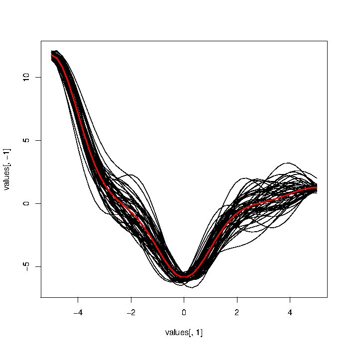
Ok, here is the answer i came up with (it's essentially taken from here and here). The idea is to project some random pairs $\{x_i,y_i\}$ unto a spline basis. Then, we are assured to get a draw from a (smooth) GP.

require("MASS")
calcSigma<-function(X1,X2,l=1){
    Sigma<-matrix(rep(0,length(X1)*length(X2)),nrow=length(X1))
    for(i in 1:nrow(Sigma)){
        for (j in 1:ncol(Sigma)) Sigma[i,j]<-exp(-1/2*(abs(X1[i]-X2[j])/l)^2)
    }
    return(Sigma)
}
# The standard deviation of the noise
n.samples<-50
n.draws<-50
x.star<-seq(-5,5,len=n.draws)
nval<-3
f<-data.frame(x=seq(-5,5,l=nval),y=rnorm(nval,0,10))
sigma.n<-0.2
# Recalculate the mean and covariance functions
k.xx<-calcSigma(f$x,f$x)
k.xxs<-calcSigma(f$x,x.star)
k.xsx<-calcSigma(x.star,f$x)
k.xsxs<-calcSigma(x.star,x.star)
f.bar.star<-k.xsx%*%solve(k.xx+sigma.n^2*diag(1,ncol(k.xx)))%*%f$y
cov.f.star<-k.xsxs-k.xsx%*%solve(k.xx+sigma.n^2*diag(1,ncol(k.xx)))%*%k.xxs
values<-matrix(rep(0,length(x.star)*n.samples),ncol=n.samples)
for (i in 1:n.samples)  values[,i]<-mvrnorm(1,f.bar.star,cov.f.star)
values<-cbind(x=x.star,as.data.frame(values))
matplot(x=values[,1],y=values[,-1],lty=1,type="l",col="black")
lines(x.star,f.bar.star,col="red",lwd=2)

A trial. Smooth functions

$\endgroup$
0

Your Answer

By clicking “Post Your Answer”, you agree to our terms of service and acknowledge you have read our privacy policy.

Not the answer you're looking for? Browse other questions tagged or ask your own question.