Why am I beating Bayes error rate in this simulation?

Question

I am trying to recreate Figure 2.4 from Elements of Statistical Learning, which shows the training error rate, test error rate, and optimal Bayes error rate for binary classification using $k$-nearest neighbors for various values of $k$ in $[1,150]$. The problem is, my test error rates are way too low and are below the Bayes error rate.

The data is generated hierarchically as follows. For group A, ten means $m_k$ are drawn from $N_2((1,0)',I_2)$. Observations are drawn by choosing a mean $m_k$ uniformly at random from $\{m_1,\dotsc,m_{10}\}$, and drawing the observation from $N_2(m_k, I_2/5)$. For group B, the means are drawn from $N_2((0,1)',I_2)$ instead of $N_2((1,0)',I_2)$.

Here is my code for generating training and test data:

library(MASS)  # for mvn sampling "mvrnorm"
library(class) # for k-nearest neighbors "knn"

set.seed(1000)

meansA = mvrnorm(10,c(1,0),diag(rep(1,2)))
meansB = mvrnorm(10,c(0,1),diag(rep(1,2)))
trainingAhidden = sample(10,100,TRUE)
trainingBhidden = sample(10,100,TRUE)
testAhidden = sample(10,5000,TRUE)
testBhidden = sample(10,5000,TRUE)
trainingAdata = t(sapply(trainingAhidden,function(x) mvrnorm(1,meansA[x,],diag(rep(1,2)/5))))
trainingBdata = t(sapply(trainingBhidden,function(x) mvrnorm(1,meansB[x,],diag(rep(1,2)/5))))
testAdata = t(sapply(testAhidden,function(x) mvrnorm(1,meansA[x,],diag(rep(1,2)/5))))
testBdata = t(sapply(testBhidden,function(x) mvrnorm(1,meansB[x,],diag(rep(1,2)/5))))
trainingY = gl(2,100,200)
testY = gl(2,5000,10000)
training = list(X = rbind(trainingAdata,trainingBdata),Y = trainingY)
test = list(X = rbind(testAdata,testBdata), Y = testY)

Even 9-nearest neighbors gives a test error rate of 0.1388, way below the optimal Bayes error rate of 0.21 given in the book:

> results = knn(training$X,test$X,training$Y,k=9)
> tab = table(results,test$Y)
1 - sum(diag(tab))/sum(tab)
[1] 0.1388

What have I done wrong?

Answer 1

The Bayes error rate depends on the particular collection of $m_k$ for the groups A and B.

In your specific case the Bayes error rate is about 0.12

CODE EXAMPLE TO CALCULATE BAYES ERROR RATE

# calculating the theoretic distributions on a grid
za <- matrix(rep(0,100*100),100)
zb <- matrix(rep(0,100*100),100)
x <- seq(-4,5,length.out=100)
y <- seq(-4,5,length.out=100)
for (i in 1:100) {
  for (j in 1:100) {
    for (k in 1:10)
    {
      za[i,j] <- za[i,j]+0.1*dmvnorm(c(x[i],y[j]),meansA[k,],diag(rep(1,2)/5))
      zb[i,j] <- zb[i,j]+0.1*dmvnorm(c(x[i],y[j]),meansB[k,],diag(rep(1,2)/5))
    }
  }
}


# doing the integration to obtain the bayes error rate
dx=x[2]-x[1]
dy=y[2]-y[1]
bayes=0

for (i in 1:100) {
  for (j in 1:100) {
    bayes = bayes + 0.5*max(za[i,j],zb[i,j])*dx*dy
  }
}
1 - sum(diag(tab))/sum(tab)
1- bayes

# plotting the knn result with the bayes classifier
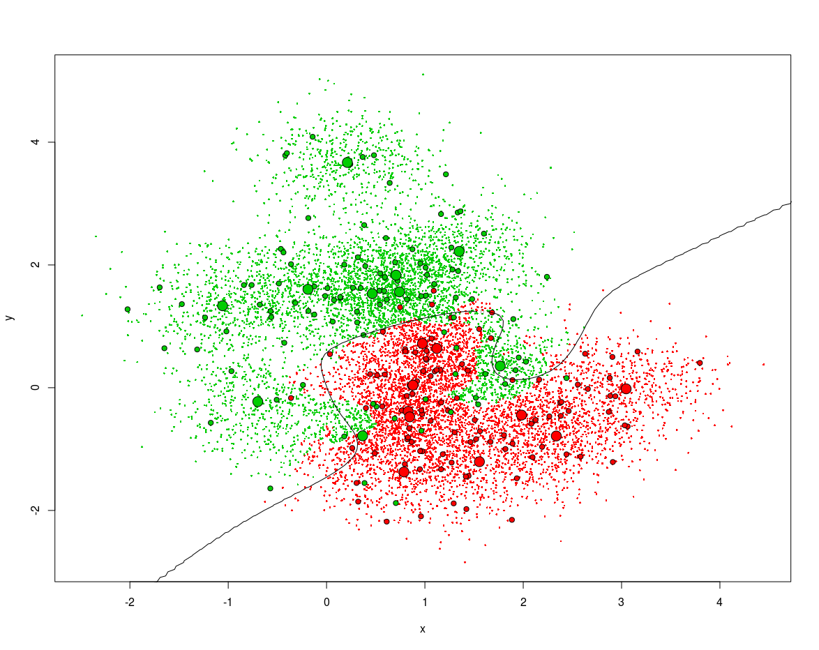
plot(test$X,pch=21,col=alpha(c(2,3)[results],0),bg=alpha(c(2,3)[results],1),cex=0.4,xlab="x",ylab="y")
points(training$X,pch=21,col=1,bg=c(2,3)[training$Y])
points(meansA,col=1,pch=21,bg=2,cex=2)
points(meansB,col=1,pch=21,bg=3,cex=2)
contour(x,y,za-zb,level=0,col=1,add=1)


# plotting the theoretic distributions with the bayes classifier
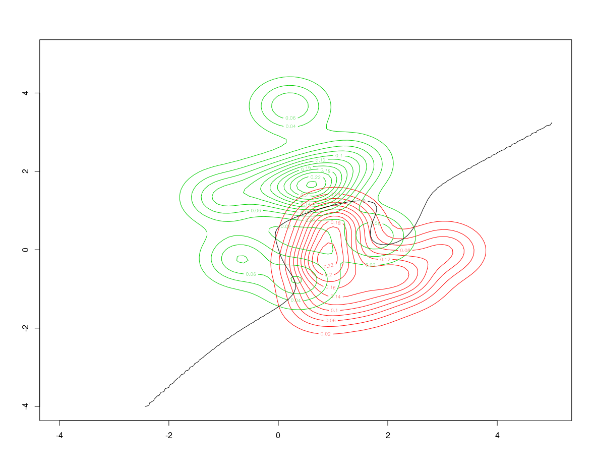
contour(x,y,za,add=0,col=2)
contour(x,y,zb,add=1,col=3)
contour(x,y,za-zb,level=0,col=1,add=1)

OUTPUT PLOTS

Contours of distributions for class A and B and Bayes classifier which is at values $p(x \vert A) = p(x \vert B)$. The overlap with the specific means (which is different for your example compared to the book) determines the error rate.

results of your 9 nearest neighbours classification. small points are the classified test sample, medium points are the training sample, big points are the 10 means for each class