Basic preconditioned gradient descent example

Question

I'm exploring preconditioned gradient descent using a similar toy problem described in the first part of Lecture 8: Accelerating SGD with preconditioning and adaptive learning rates.

I have the function $f(x,y) = x^2 + 10\,y^2$ which has a gradient of $[2x, 20y]$.

I know the ideal form of the function is $f(x,y) = x^2 + y^2$ which has a gradient of $[2\,x, 2\,y]$.

How do I solve for the precondition matrix in the equation, $w_{t+1} = w_t - \alpha\,P\,\nabla f(w_t)$, like the first activity box asks? In this case $P$ would just be $[1, \frac{1}{10}]$?

At the bottom of the second page it says:

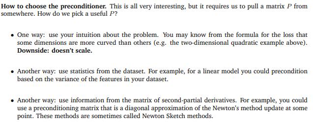
I'm having trouble understanding how to formally solve for it in variance context described in the answer here Preconditioning gradient descent. I also see in that answer, reference of the third approach w/ $P = [H f(x^*)]^{-1}$.

I am unable to find any other examples walked through online.

Answer 1

Since the hessian is constant $P = H^{-1}$ is optimal (you fully recover Newton's method): $P = H^{-1} = \text{diag}(1/2, 1/20)$. This is equivalent to making the change of variables $x = \frac{1}{\sqrt{2}} x'$ and $y = \frac{1}{\sqrt{20}} y'$ which gives you the desired $\frac{1}{2} (x'^2 + y'^2)$ form.

As for approach 2, this is just a systematic way of estimating the scale of your variables. Get an empirical estimate for the covariance matrix $\Sigma \approx \text{Cov}(x)$. The answer you referenced shows how $P = \Sigma$ follows from a change of variable and chain-rule.

What distribution do you sample if you want to do approach 2? If you treat your objective function as a negative log-likelihood, then you should be sampling from a normal distribution with $\frac{1}{2} \Sigma^{-1} = \operatorname{diag}(1, 10)$. So you should get $\Sigma = \operatorname{diag}(1/2, 1/20)$. If you were to take many random samples from this distribution and calculate their covariance, you would get the same answer since $\Sigma_{i,j} := \operatorname{E} [(x_i - \mu_i)( x_j - \mu_j)] = \operatorname{Cov}(x)$ (see wikipedia).

These approaches are equivalent when your data is normally-distributed and you have a lot of it. In practice, approach 2 is more generally applicable to situations where the Hessian is not constant, but can be somewhat crude.

Automatically computing a dynamic preconditioning matrix is a very well studied topic. Optimization methods that do this are called Quasi-Newton methods.

Answer 2

I'm fairly sure you can just use the Hessian, which in this case is $$ 2\begin{bmatrix} 1 & 0\\ 0 & 10 \end{bmatrix} $$

This comes from method 3 (using second-partial derivative information), and possibly also method 1.

The reason we're using the exact matrix here instead of an approximation is because this is a simple case; as noted elsewhere efficiency can be an issue with larger dimensions.

We've already got a diagonal matrix, so even if we did approximate as suggested it would be the same. Note this matrix also satisfies the criteria of being symmetric and positive semi-definite.

Answer 3

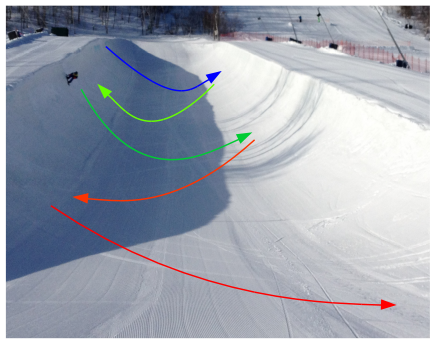
This is the problem that preconditioning tries to solve:

From this blog (also discussed here on stackexchange: Fitting SIR model with 2019-nCoV data doesn't conververge)

Problems:

• With gradient descent methods you follow a path down-hill. But, your algorithm is often not as smooth as water and doesn't flow straight down in the most efficient way. Instead, often the algorithm will 'over-shoot' and follow an (inefficient) zigzag path.
• Another problem is that the algorithm might have some basic rules to decide when to stop. For instance, deciding to stop when the step sizes are getting very small. However, for that stopping rule, when you are not looking into the direction of the optimum (because you are looking along the slow zigzag path), it might be that your step sizes are small while the optimum is still far away.

(the first problem is about the speed of getting a solution/convergence, the second problem is about the accuracy of the result)

Methods to 'pre-condition':

So it would be nice if you could change the scale of the different variables somehow (make them more equal instead of having this valley). You only need to know how.

• method 1: use the formula for the problem or some intuition about the problem.

  In your case, the function $f(x,y) = x^2 + 10y^2$, you can compute the scaling/pre-conditioning based on the formula. In the formulation of your reference... $P$ should be a matrix. That is $P$ is not $\left[1,1/10\right]$ but instead $$P = \begin{bmatrix} 1 & 0 \\ 0 & 1/10 \end{bmatrix}$$ It is the scaling of the variables that is a vector, namely $R = \left[1,\sqrt{1/10}\right]$.

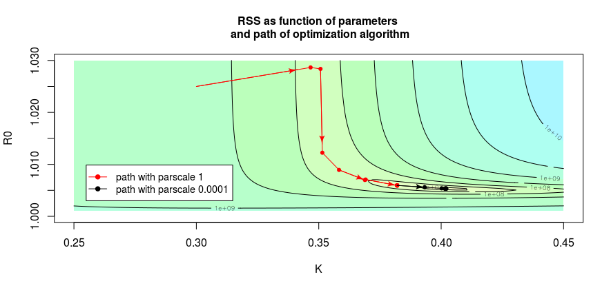
  Without formula, you can use 'intuition'. For instance, you might be having features with widely varying scales. I often just do this. Scale the variables such that the range of the 'expected' solution will be similar for each variable. (In the image below you see this as well. The range of the $R_0$ and $K$ parameter is a lot different)

• method 2: Use the data/variance. I believe that this refers to using a sample distribution of the features (or some other information about the scale of spread). The variance of the features relates to the curvature of the likelihood function (observed information matrix). Maybe this method is also much the same as 'use intuition'.

  Aside from just looking at the scale of the parameters, it is also important to look at the 'variation'. If some parameter is around $1 \, kilometer \pm 0.001 \, kilometer$, then the loss function has more curvature than a parameter around $10 \, meter \pm 2 \, meter$. (you can see this in the image below, the parameter $R_0 \approx 1$ has a larger scale than the $K \approx 0.4$ parameter, but the variation is in a much smaller range)

• method 3: You may not have a formula or intuition like in method 1, but you could compute the Hessian at some point during the descent and adapt the scaling accordingly.

  This method 3 is particularly nice if the problem is not continuous. For instance in the image below you get that the hessian and the scale is varying. Intuitively, the line that the "half-pipe" follows is bended (in the beginning the $K$ parameter has more curvature, but later the $R_0$ parameter). In these cases you can not easily solve problems of convergence by just setting a (single) pre-conditioning from the start, and you need to change it in multiple steps (along the path).