This question arose from this question.
EDIT 1:
Forgot to include an error term in the example.
EDIT 2:
The model I am trying to fit is $y = \sin(x) + \epsilon_i$.
Given a certain data set, according to R I should get $\hat{y} = 0.60330 + 0.01797x$:
set.seed(1234)

 n <- 5
 df <- data.frame(x=runif(n, 1, 10))
 df$mean.y.given.x <- sin(df$x)
 df$y <- df$mean.y.given.x + rnorm(n)
 model <- lm(y ~ x, data=df)
 summary(model)

 Call:
 lm(formula = y ~ x, data = df)

 Residuals:
     1       2       3       4       5
 0.6190 -1.1402 -0.4852 -0.2877  1.2941

 Coefficients:
              Estimate Std. Error t value Pr(>|t|)
 (Intercept)  0.60330    1.45534   0.415    0.706
 x            0.01797    0.22460   0.080    0.941

 Residual standard error: 1.107 on 3 degrees of freedom
 Multiple R-squared:  0.00213,  Adjusted R-squared:  -0.3305
 F-statistic: 0.006404 on 1 and 3 DF,  p-value: 0.9413
I would like to obtain $\hat{y}$ by hand now. However, all the questions I have done thus far is always of the form $y_i = \alpha + \beta x$, where $\alpha$ and $\beta$ are constants, so that $y_i$ is a linear function of $x_i$. Therefore, I am unsure of how to proceed when $y_i$ is not a linear function of $x$, hence my request for a worked examples for these kind of questions.
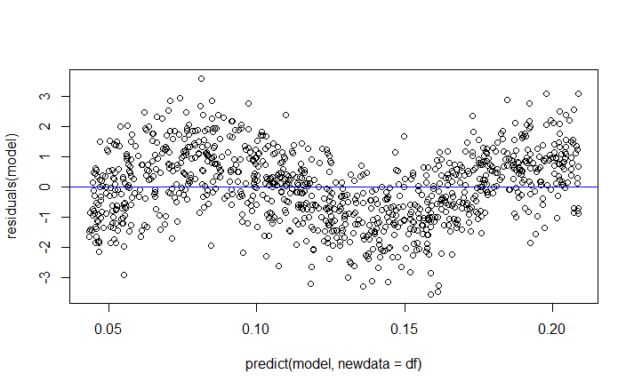
After that, I expect to be able to show that $E(y_i-\hat{y_i}) \neq 0$ because the plot of the residuals against the predicted value (for large $n$) is:
set.seed(1234)
n <- 1000
df <- data.frame(x=runif(n, 1, 10))
df$mean.y.given.x <- sin(df$x)
df$y <- df$mean.y.given.x + rnorm(n)
model <- lm(y ~ x, data=df)
plot(predict(model, newdata=df), residuals(model))
abline(a=0,b=0,col='blue')
 Based on the above plot, $E(y_i-\hat{y_i}) \neq 0$ must be true in this case, right?