replaced http://stats.stackexchange.com/ with https://stats.stackexchange.com/
Source Link

There's a very straightforward means by which to use almost any correlation measure to fit linear regressions, and which reproduces least squares when you use the Pearson correlation.

Consider that if the slope of a relationship is $\beta$, the correlation between $y-\beta x$ and $x$ should be expected to be $0$.

Indeed, if it were anything other than $0$, there'd be some uncaptured linear relationship - which is what the correlation measure would be picking up.

We might therefore estimate the slope by finding the slope, $\tilde{\beta}$ that makes the sample correlation between $y-\tilde{\beta} x$ and $x$ be $0$. In many cases -- e.g. when using rank-based measures -- the correlation will be a step-function of the value of the slope estimate, so there may be an interval where it's zero. In that case we normally define the sample estimate to be the center of the interval. Often the step function jumps from above zero to below zero at some point, and in that case the estimate is at the jump point.

This definition works, for example, with all manner of rank based and robust correlations. It can also be used to obtain an interval for the slope (in the usual manner - by finding the slopes that mark the border between just significant correlations and just insignificant correlations).

This only defines the slope, of course; once the slope is estimated, the intercept can be based on a suitable location estimate computed on the residuals $y-\tilde{\beta}x$. With the rank-based correlations the median is a common choice, but there are many other suitable choices.

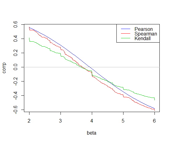
Here's the correlation plotted against the slope for the car data in R:
enter image description here

The Pearson correlation crosses 0 at the least squares slope, 3.932
The Kendall correlation crosses 0 at the Theil-Sen slope, 3.667
The Spearman correlation crosses 0 giving a "Spearman-line" slope of 3.714

Those are the three slope estimates for our example. Now we need intercepts. For simplicity I'll just use the mean residual for the first intercept and the median for the other two (it doesn't matter very much in this case):

           intercept
 Pearson:  -17.573 *     
 Kendall:  -15.667
 Spearman: -16.285

*(the small difference from least squares is due to rounding error in the slope estimate; no doubt there's similar rounding error in the other estimates)

The corresponding fitted lines (using the same color scheme as above) are:

enter image description here

Edit: By comparison, the quadrant-correlation slope is 3.333

Both the Kendall correlation and Spearman correlation slopes are substantially more robust to influential outliers than least squares. See herehere for a dramatic example in the case of the Kendall.

There's a very straightforward means by which to use almost any correlation measure to fit linear regressions, and which reproduces least squares when you use the Pearson correlation.

Consider that if the slope of a relationship is $\beta$, the correlation between $y-\beta x$ and $x$ should be expected to be $0$.

Indeed, if it were anything other than $0$, there'd be some uncaptured linear relationship - which is what the correlation measure would be picking up.

We might therefore estimate the slope by finding the slope, $\tilde{\beta}$ that makes the sample correlation between $y-\tilde{\beta} x$ and $x$ be $0$. In many cases -- e.g. when using rank-based measures -- the correlation will be a step-function of the value of the slope estimate, so there may be an interval where it's zero. In that case we normally define the sample estimate to be the center of the interval. Often the step function jumps from above zero to below zero at some point, and in that case the estimate is at the jump point.

This definition works, for example, with all manner of rank based and robust correlations. It can also be used to obtain an interval for the slope (in the usual manner - by finding the slopes that mark the border between just significant correlations and just insignificant correlations).

This only defines the slope, of course; once the slope is estimated, the intercept can be based on a suitable location estimate computed on the residuals $y-\tilde{\beta}x$. With the rank-based correlations the median is a common choice, but there are many other suitable choices.

Here's the correlation plotted against the slope for the car data in R:

enter image description here

The Pearson correlation crosses 0 at the least squares slope, 3.932
The Kendall correlation crosses 0 at the Theil-Sen slope, 3.667
The Spearman correlation crosses 0 giving a "Spearman-line" slope of 3.714

Those are the three slope estimates for our example. Now we need intercepts. For simplicity I'll just use the mean residual for the first intercept and the median for the other two (it doesn't matter very much in this case):

           intercept
 Pearson:  -17.573 *     
 Kendall:  -15.667
 Spearman: -16.285

*(the small difference from least squares is due to rounding error in the slope estimate; no doubt there's similar rounding error in the other estimates)

The corresponding fitted lines (using the same color scheme as above) are:

enter image description here

Edit: By comparison, the quadrant-correlation slope is 3.333

Both the Kendall correlation and Spearman correlation slopes are substantially more robust to influential outliers than least squares. See here for a dramatic example in the case of the Kendall.

Bounty Ended with 50 reputation awarded by Firebug
inserted missing "x" character into residual definition
Source Link
Glen_b
  • 290.5k
  • 37
  • 652
  • 1.1k

There's a very straightforward means by which to use almost any correlation measure to fit linear regressions, and which reproduces least squares when you use the Pearson correlation.

Consider that if the slope of a relationship is $\beta$, the correlation between $y-\beta x$ and $x$ should be expected to be $0$.

Indeed, if it were anything other than $0$, there'd be some uncaptured linear relationship - which is what the correlation measure would be picking up.

We might therefore estimate the slope by finding the slope, $\tilde{\beta}$ that makes the sample correlation between $y-\tilde{\beta} x$ and $x$ be $0$. In many cases -- e.g. when using rank-based measures -- the correlation will be a step-function of the value of the slope estimate, so there may be an interval where it's zero. In that case we normally define the sample estimate to be the center of the interval. Often the step function jumps from above zero to below zero at some point, and in that case the estimate is at the jump point.

This definition works, for example, with all manner of rank based and robust correlations. It can also be used to obtain an interval for the slope (in the usual manner - by finding the slopes that mark the border between just significant correlations and just insignificant correlations).

This only defines the slope, of course; once the slope is estimated, the intercept can be based on a suitable location estimate computed on the residuals $y-\tilde{\beta}$$y-\tilde{\beta}x$. With the rank-based correlations the median is a common choice, but there are many other suitable choices.

Here's the correlation plotted against the slope for the car data in R:

enter image description here

The Pearson correlation crosses 0 at the least squares slope, 3.932
The Kendall correlation crosses 0 at the Theil-Sen slope, 3.667
The Spearman correlation crosses 0 giving a "Spearman-line" slope of 3.714

Those are the three slope estimates for our example. Now we need intercepts. For simplicity I'll just use the mean residual for the first intercept and the median for the other two (it doesn't matter very much in this case):

           intercept
 Pearson:  -17.573 *     
 Kendall:  -15.667
 Spearman: -16.285

*(the small difference from least squares is due to rounding error in the slope estimate; no doubt there's similar rounding error in the other estimates)

The corresponding fitted lines (using the same color scheme as above) are:

enter image description here

Edit: By comparison, the quadrant-correlation slope is 3.333

Both the Kendall correlation and Spearman correlation slopes are substantially more robust to influential outliers than least squares. See here for a dramatic example in the case of the Kendall.

There's a very straightforward means by which to use almost any correlation measure to fit linear regressions, and which reproduces least squares when you use the Pearson correlation.

Consider that if the slope of a relationship is $\beta$, the correlation between $y-\beta x$ and $x$ should be expected to be $0$.

Indeed, if it were anything other than $0$, there'd be some uncaptured linear relationship - which is what the correlation measure would be picking up.

We might therefore estimate the slope by finding the slope, $\tilde{\beta}$ that makes the sample correlation between $y-\tilde{\beta} x$ and $x$ be $0$. In many cases -- e.g. when using rank-based measures -- the correlation will be a step-function of the value of the slope estimate, so there may be an interval where it's zero. In that case we normally define the sample estimate to be the center of the interval. Often the step function jumps from above zero to below zero at some point, and in that case the estimate is at the jump point.

This definition works, for example, with all manner of rank based and robust correlations. It can also be used to obtain an interval for the slope (in the usual manner - by finding the slopes that mark the border between just significant correlations and just insignificant correlations).

This only defines the slope, of course; once the slope is estimated, the intercept can be based on a suitable location estimate computed on the residuals $y-\tilde{\beta}$. With the rank-based correlations the median is a common choice, but there are many other suitable choices.

Here's the correlation plotted against the slope for the car data in R:

enter image description here

The Pearson correlation crosses 0 at the least squares slope, 3.932
The Kendall correlation crosses 0 at the Theil-Sen slope, 3.667
The Spearman correlation crosses 0 giving a "Spearman-line" slope of 3.714

Those are the three slope estimates for our example. Now we need intercepts. For simplicity I'll just use the mean residual for the first intercept and the median for the other two (it doesn't matter very much in this case):

           intercept
 Pearson:  -17.573 *     
 Kendall:  -15.667
 Spearman: -16.285

*(the small difference from least squares is due to rounding error in the slope estimate; no doubt there's similar rounding error in the other estimates)

The corresponding fitted lines (using the same color scheme as above) are:

enter image description here

Edit: By comparison, the quadrant-correlation slope is 3.333

Both the Kendall correlation and Spearman correlation slopes are substantially more robust to influential outliers than least squares. See here for a dramatic example in the case of the Kendall.

There's a very straightforward means by which to use almost any correlation measure to fit linear regressions, and which reproduces least squares when you use the Pearson correlation.

Consider that if the slope of a relationship is $\beta$, the correlation between $y-\beta x$ and $x$ should be expected to be $0$.

Indeed, if it were anything other than $0$, there'd be some uncaptured linear relationship - which is what the correlation measure would be picking up.

We might therefore estimate the slope by finding the slope, $\tilde{\beta}$ that makes the sample correlation between $y-\tilde{\beta} x$ and $x$ be $0$. In many cases -- e.g. when using rank-based measures -- the correlation will be a step-function of the value of the slope estimate, so there may be an interval where it's zero. In that case we normally define the sample estimate to be the center of the interval. Often the step function jumps from above zero to below zero at some point, and in that case the estimate is at the jump point.

This definition works, for example, with all manner of rank based and robust correlations. It can also be used to obtain an interval for the slope (in the usual manner - by finding the slopes that mark the border between just significant correlations and just insignificant correlations).

This only defines the slope, of course; once the slope is estimated, the intercept can be based on a suitable location estimate computed on the residuals $y-\tilde{\beta}x$. With the rank-based correlations the median is a common choice, but there are many other suitable choices.

Here's the correlation plotted against the slope for the car data in R:

enter image description here

The Pearson correlation crosses 0 at the least squares slope, 3.932
The Kendall correlation crosses 0 at the Theil-Sen slope, 3.667
The Spearman correlation crosses 0 giving a "Spearman-line" slope of 3.714

Those are the three slope estimates for our example. Now we need intercepts. For simplicity I'll just use the mean residual for the first intercept and the median for the other two (it doesn't matter very much in this case):

           intercept
 Pearson:  -17.573 *     
 Kendall:  -15.667
 Spearman: -16.285

*(the small difference from least squares is due to rounding error in the slope estimate; no doubt there's similar rounding error in the other estimates)

The corresponding fitted lines (using the same color scheme as above) are:

enter image description here

Edit: By comparison, the quadrant-correlation slope is 3.333

Both the Kendall correlation and Spearman correlation slopes are substantially more robust to influential outliers than least squares. See here for a dramatic example in the case of the Kendall.

fixed minor formatting issue
Source Link
Glen_b
  • 290.5k
  • 37
  • 652
  • 1.1k

There's a very straightforward means by which to use almost any correlation measure to fit linear regressions, and which reproduces least squares when you use the Pearson correlation.

Consider that if the slope of a relationship is $\beta$, the correlation between $y-\beta x$ and $x$ should be expected to be $0$.

Indeed, if it were anything other than $0$, there'd be some uncaptured linear relationship - which is what the correlation measure would be picking up.

We might therefore estimate the slope by finding the slope, $\tilde{\beta}$ that makes the sample correlation between $y-\tilde{\beta} x$ and $x$ be $0$. In many cases -- e.g. when using rank-based measures -- the correlation will be a step-function of the value of the slope estimate, so there may be an interval where it's zero. In that case we normally define the sample estimate to be the center of the interval. Often the step function jumps from above zero to below zero at some point, and in that case the estimate is at the jump point.

This definition works, for example, with all manner of rank based and robust correlations. It can also be used to obtain an interval for the slope (in the usual manner - by finding the slopes that mark the border between just significant correlations and just insignificant correlations).

This only defines the slope, of course; once the slope is estimated, the intercept can be based on a suitable location estimate computed on the residuals $y-\tilde{\beta}$. With the rank-based correlations the median is a common choice, but there are many other suitable choices.

Here's the correlation plotted against the slope for the car data in R:

enter image description here

The Pearson correlation crosses 0 at the least squares slope, 3.932
The Kendall correlation crosses 0 at the Theil-Sen slope, 3.667
The Spearman correlation crosses 0 giving a "Spearman-line" slope of 3.714

Those are the three slope estimates for our example. Now we need intercepts. For simplicity I'll just use the mean residual for the first intercept and the median for the other two (it doesn't matter very much in this case):

           intercept
 Pearson:  -17.573\*573 *     
 Kendall:  -15.667
 Spearman: -16.285

*(the small difference from least squares is due to rounding error in the slope estimate; no doubt there's similar rounding error in the other estimates)

The corresponding fitted lines (using the same color scheme as above) are:

enter image description here

Edit: By comparison, the quadrant-correlation slope is 3.333

Both the Kendall correlation and Spearman correlation slopes are substantially more robust to influential outliers than least squares. See here for a dramatic example in the case of the Kendall.

There's a very straightforward means by which to use almost any correlation measure to fit linear regressions, and which reproduces least squares when you use the Pearson correlation.

Consider that if the slope of a relationship is $\beta$, the correlation between $y-\beta x$ and $x$ should be expected to be $0$.

Indeed, if it were anything other than $0$, there'd be some uncaptured linear relationship - which is what the correlation measure would be picking up.

We might therefore estimate the slope by finding the slope, $\tilde{\beta}$ that makes the sample correlation between $y-\tilde{\beta} x$ and $x$ be $0$. In many cases -- e.g. when using rank-based measures -- the correlation will be a step-function of the value of the slope estimate, so there may be an interval where it's zero. In that case we normally define the sample estimate to be the center of the interval. Often the step function jumps from above zero to below zero at some point, and in that case the estimate is at the jump point.

This definition works, for example, with all manner of rank based and robust correlations. It can also be used to obtain an interval for the slope (in the usual manner - by finding the slopes that mark the border between just significant correlations and just insignificant correlations).

This only defines the slope, of course; once the slope is estimated, the intercept can be based on a suitable location estimate computed on the residuals $y-\tilde{\beta}$. With the rank-based correlations the median is a common choice, but there are many other suitable choices.

Here's the correlation plotted against the slope for the car data in R:

enter image description here

The Pearson correlation crosses 0 at the least squares slope, 3.932
The Kendall correlation crosses 0 at the Theil-Sen slope, 3.667
The Spearman correlation crosses 0 giving a "Spearman-line" slope of 3.714

Those are the three slope estimates for our example. Now we need intercepts. For simplicity I'll just use the mean residual for the first intercept and the median for the other two (it doesn't matter very much in this case):

           intercept
 Pearson:  -17.573\*     
 Kendall:  -15.667
 Spearman: -16.285

*(the small difference from least squares is due to rounding error in the slope estimate; no doubt there's similar rounding error in the other estimates)

The corresponding fitted lines (using the same color scheme as above) are:

enter image description here

Edit: By comparison, the quadrant-correlation slope is 3.333

Both the Kendall correlation and Spearman correlation slopes are substantially more robust to influential outliers than least squares. See here for a dramatic example in the case of the Kendall.

There's a very straightforward means by which to use almost any correlation measure to fit linear regressions, and which reproduces least squares when you use the Pearson correlation.

Consider that if the slope of a relationship is $\beta$, the correlation between $y-\beta x$ and $x$ should be expected to be $0$.

Indeed, if it were anything other than $0$, there'd be some uncaptured linear relationship - which is what the correlation measure would be picking up.

We might therefore estimate the slope by finding the slope, $\tilde{\beta}$ that makes the sample correlation between $y-\tilde{\beta} x$ and $x$ be $0$. In many cases -- e.g. when using rank-based measures -- the correlation will be a step-function of the value of the slope estimate, so there may be an interval where it's zero. In that case we normally define the sample estimate to be the center of the interval. Often the step function jumps from above zero to below zero at some point, and in that case the estimate is at the jump point.

This definition works, for example, with all manner of rank based and robust correlations. It can also be used to obtain an interval for the slope (in the usual manner - by finding the slopes that mark the border between just significant correlations and just insignificant correlations).

This only defines the slope, of course; once the slope is estimated, the intercept can be based on a suitable location estimate computed on the residuals $y-\tilde{\beta}$. With the rank-based correlations the median is a common choice, but there are many other suitable choices.

Here's the correlation plotted against the slope for the car data in R:

enter image description here

The Pearson correlation crosses 0 at the least squares slope, 3.932
The Kendall correlation crosses 0 at the Theil-Sen slope, 3.667
The Spearman correlation crosses 0 giving a "Spearman-line" slope of 3.714

Those are the three slope estimates for our example. Now we need intercepts. For simplicity I'll just use the mean residual for the first intercept and the median for the other two (it doesn't matter very much in this case):

           intercept
 Pearson:  -17.573 *     
 Kendall:  -15.667
 Spearman: -16.285

*(the small difference from least squares is due to rounding error in the slope estimate; no doubt there's similar rounding error in the other estimates)

The corresponding fitted lines (using the same color scheme as above) are:

enter image description here

Edit: By comparison, the quadrant-correlation slope is 3.333

Both the Kendall correlation and Spearman correlation slopes are substantially more robust to influential outliers than least squares. See here for a dramatic example in the case of the Kendall.

added 8 characters in body
Source Link
Glen_b
  • 290.5k
  • 37
  • 652
  • 1.1k
Loading
added 8 characters in body
Source Link
Glen_b
  • 290.5k
  • 37
  • 652
  • 1.1k
Loading
added 112 characters in body
Source Link
Glen_b
  • 290.5k
  • 37
  • 652
  • 1.1k
Loading
Source Link
Glen_b
  • 290.5k
  • 37
  • 652
  • 1.1k
Loading