Added graph and sample data.
Source Link
Erik P.
  • 2k
  • 17
  • 18

I like @whuber's answer very much; it's likely to be very efficient and has a beautiful analysis. But it requires some deep insight with respect to this particular distribution. For situations where you don't have that insight (so for different distributions), I also like the following approach which works for all distributions where the PDF is twice differentiable and that second derivative has finitely many roots. It requires quite a bit of work to set up, but then afterwards you have an engine that works for most distributions you can throw at it.

Basically, the idea is to use a piecewise linear upper bound to the PDF which you adapt as you are doing rejection sampling. At the same time you have a piecewise linear lower bound for the PDF which prevents you from having to evaluate the PDF too frequently. The upper and lower bounds are given by chords and tangents to the PDF graph. The initial division into intervals is such that on each interval, the PDF is either all concave or all convex; whenever you have to reject a point (x, y) you subdivide that interval at x. (You can also do an extra subdivision at x if you had to compute the PDF because the lower bound is really bad.) This makes the subdivisions occur especially frequently where the upper (and lower) bounds are bad, so you get a really good approximation of your PDF essentially for free. The details are a little tricky to get right, but I've tried to explain most of them in this series of blog posts - especially the last one.

Those posts don't discuss what to do if the PDF is unbounded either in domain or in values; I'd recommend the somewhat obvious solution of either doing a transformation that makes them finite (which would be hard to automate) or using a cutoff. I would choose the cutoff depending on the total number of points you expect to generate, say N, and choose the cutoff so that the removed part has less than $1 / (10 N)$ probability. (This is easy enough if you have a closed form for the CDF; otherwise it might also be tricky.)

This method is implemented in Maple as the default method for user-defined continuous distributions. (Full disclosure - I work for Maplesoft.)


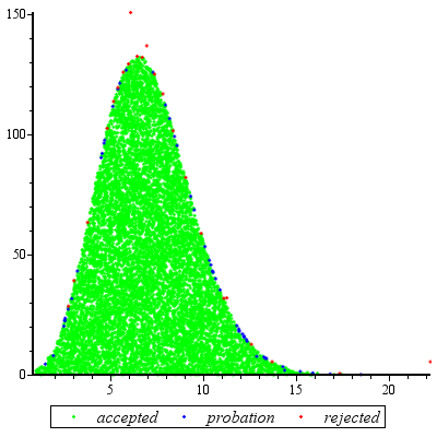
I did an example run, generating 10^4 points for c = 2, d = 3, specifying [1, 100] as the initial range for the values:
graph

There were 23 rejections (in red), 51 points "on probation" which were at the time in between the lower bound and the actual PDF, and 9949 points which were accepted after checking only linear inequalities. That's 74 evaluations of the PDF in total, or about one PDF evaluation per 135 points. The ratio should get better as you generate more points, since the approximation gets better and better (and conversely, if you generate only few points, the ratio is worse).

I like @whuber's answer very much; it's likely to be very efficient and has a beautiful analysis. But it requires some deep insight with respect to this particular distribution. For situations where you don't have that insight (so for different distributions), I also like the following approach which works for all distributions where the PDF is twice differentiable and that second derivative has finitely many roots. It requires quite a bit of work to set up, but then afterwards you have an engine that works for most distributions you can throw at it.

Basically, the idea is to use a piecewise linear upper bound to the PDF which you adapt as you are doing rejection sampling. At the same time you have a piecewise linear lower bound for the PDF which prevents you from having to evaluate the PDF too frequently. The upper and lower bounds are given by chords and tangents to the PDF graph. The initial division into intervals is such that on each interval, the PDF is either all concave or all convex; whenever you have to reject a point (x, y) you subdivide that interval at x. (You can also do an extra subdivision at x if you had to compute the PDF because the lower bound is really bad.) This makes the subdivisions occur especially frequently where the upper (and lower) bounds are bad, so you get a really good approximation of your PDF essentially for free. The details are a little tricky to get right, but I've tried to explain most of them in this series of blog posts - especially the last one.

Those posts don't discuss what to do if the PDF is unbounded either in domain or in values; I'd recommend the somewhat obvious solution of either doing a transformation that makes them finite (which would be hard to automate) or using a cutoff. I would choose the cutoff depending on the total number of points you expect to generate, say N, and choose the cutoff so that the removed part has less than $1 / (10 N)$ probability. (This is easy enough if you have a closed form for the CDF; otherwise it might also be tricky.)

This method is implemented in Maple as the default method for user-defined continuous distributions. (Full disclosure - I work for Maplesoft.)


I did an example run, generating 10^4 points for c = 2, d = 3, specifying [1, 100] as the initial range for the values:

graph

There were 23 rejections (in red), 51 points "on probation" which were at the time in between the lower bound and the actual PDF, and 9949 points which were accepted after checking only linear inequalities. That's 74 evaluations of the PDF in total, or about one PDF evaluation per 135 points. The ratio should get better as you generate more points, since the approximation gets better and better (and conversely, if you generate only few points, the ratio is worse).

Source Link
Erik P.
  • 2k
  • 17
  • 18

I like @whuber's answer very much; it's likely to be very efficient and has a beautiful analysis. But it requires some deep insight with respect to this particular distribution. For situations where you don't have that insight (so for different distributions), I also like the following approach which works for all distributions where the PDF is twice differentiable and that second derivative has finitely many roots. It requires quite a bit of work to set up, but then afterwards you have an engine that works for most distributions you can throw at it.

Basically, the idea is to use a piecewise linear upper bound to the PDF which you adapt as you are doing rejection sampling. At the same time you have a piecewise linear lower bound for the PDF which prevents you from having to evaluate the PDF too frequently. The upper and lower bounds are given by chords and tangents to the PDF graph. The initial division into intervals is such that on each interval, the PDF is either all concave or all convex; whenever you have to reject a point (x, y) you subdivide that interval at x. (You can also do an extra subdivision at x if you had to compute the PDF because the lower bound is really bad.) This makes the subdivisions occur especially frequently where the upper (and lower) bounds are bad, so you get a really good approximation of your PDF essentially for free. The details are a little tricky to get right, but I've tried to explain most of them in this series of blog posts - especially the last one.

Those posts don't discuss what to do if the PDF is unbounded either in domain or in values; I'd recommend the somewhat obvious solution of either doing a transformation that makes them finite (which would be hard to automate) or using a cutoff. I would choose the cutoff depending on the total number of points you expect to generate, say N, and choose the cutoff so that the removed part has less than $1 / (10 N)$ probability. (This is easy enough if you have a closed form for the CDF; otherwise it might also be tricky.)

This method is implemented in Maple as the default method for user-defined continuous distributions. (Full disclosure - I work for Maplesoft.)