replaced http://stats.stackexchange.com/ with https://stats.stackexchange.com/
Source Link

@NickCox has presented an interesting strategy (+1). I might consider it more exploratory in nature however, due to the concern that @whuber points outpoints out.

Some people don't feel comfortable using a parametric test here (although if the assumptions hold, I don't know of any problem). One very broadly applicable technique is to use the Parametric Bootstrap Cross-fitting Method (I describe the algorithm herehere). We can try applying it to these data:

The summary statistics, and the kernel density plots for the sampling distributions show several interesting features. The log likelihood for the single component model is rarely greater than that of the two component fit, even when the true data generating process has only a single component, and when it is greater, the amount is trivial. The idea of comparing models that differ in their ability to fit data is one of the motivations behind the PBCM. The two sampling distributions barely overlap at all; only .35% of x2.d are less than the maximum x1.d value. If you selected a two component model if the difference in log likelihood were >9.7, you would incorrectly select the one component model .01% and the two component model .02% of the time. These are highly discriminable. If, on the other hand, you chose to use the one component model as a null hypothesis, your observed result is sufficiently small as not to show up in the empirical sampling distribution in 10,000 iterations. We can use the rule of 3 (see herehere) to place an upper bound on the p-value, namely, we estimate your p-value is less than .0003. That is, this is highly significant.

This raises the question of why these results diverge so much from your dip test. (To answer your explicit question, your dip test provides no evidence that there are two real modes.) I honestly don't know the dip test, so it's hard to say; it may be underpowered. However, I think the likely answer is that this approach assumes your data are generated by true normal[s]. A Shapiro-Wilk test for your data is highly significant ($p < .000001$), and it is also highly significant for the optimal Box-Cox transformation of your data (the inverse square root; $p < .001$). However, data are never really normal (cf., this famous quotethis famous quote), and the underlying components, should they exist, aren't guaranteed to be perfectly normal either. If you find it reasonable that your data could come from a positively skewed distribution, rather than a normal, this level of bimodality may well be within the typical range of variation, which is what I suspect the dip test is saying.

@NickCox has presented an interesting strategy (+1). I might consider it more exploratory in nature however, due to the concern that @whuber points out.

Some people don't feel comfortable using a parametric test here (although if the assumptions hold, I don't know of any problem). One very broadly applicable technique is to use the Parametric Bootstrap Cross-fitting Method (I describe the algorithm here). We can try applying it to these data:

The summary statistics, and the kernel density plots for the sampling distributions show several interesting features. The log likelihood for the single component model is rarely greater than that of the two component fit, even when the true data generating process has only a single component, and when it is greater, the amount is trivial. The idea of comparing models that differ in their ability to fit data is one of the motivations behind the PBCM. The two sampling distributions barely overlap at all; only .35% of x2.d are less than the maximum x1.d value. If you selected a two component model if the difference in log likelihood were >9.7, you would incorrectly select the one component model .01% and the two component model .02% of the time. These are highly discriminable. If, on the other hand, you chose to use the one component model as a null hypothesis, your observed result is sufficiently small as not to show up in the empirical sampling distribution in 10,000 iterations. We can use the rule of 3 (see here) to place an upper bound on the p-value, namely, we estimate your p-value is less than .0003. That is, this is highly significant.

This raises the question of why these results diverge so much from your dip test. (To answer your explicit question, your dip test provides no evidence that there are two real modes.) I honestly don't know the dip test, so it's hard to say; it may be underpowered. However, I think the likely answer is that this approach assumes your data are generated by true normal[s]. A Shapiro-Wilk test for your data is highly significant ($p < .000001$), and it is also highly significant for the optimal Box-Cox transformation of your data (the inverse square root; $p < .001$). However, data are never really normal (cf., this famous quote), and the underlying components, should they exist, aren't guaranteed to be perfectly normal either. If you find it reasonable that your data could come from a positively skewed distribution, rather than a normal, this level of bimodality may well be within the typical range of variation, which is what I suspect the dip test is saying.

added 241 characters in body
Source Link
gung - Reinstate Monica
  • 147.5k
  • 89
  • 406
  • 717

Let me suggest another strategy: You could fit a Gaussian finite mixture model. Note that this makes the very strong assumption that your data are drawn from one or more true normals. In R, you can use As both @whuber and @NickCox point out in the Mclust package to docomments, without a substantive interpretation of these data—supported by well-established theory—to support this assumption, this strategy should be considered exploratory as well.

Now lets fit a Gaussian finite mixture model. In R, you can use the Mclust package to do this:

Let me suggest another strategy: You could fit a Gaussian finite mixture model. Note that this makes the very strong assumption that your data are drawn from one or more true normals. In R, you can use the Mclust package to do this.

Now lets fit a Gaussian finite mixture model:

Let me suggest another strategy: You could fit a Gaussian finite mixture model. Note that this makes the very strong assumption that your data are drawn from one or more true normals. As both @whuber and @NickCox point out in the comments, without a substantive interpretation of these data—supported by well-established theory—to support this assumption, this strategy should be considered exploratory as well.

Now lets fit a Gaussian finite mixture model. In R, you can use the Mclust package to do this:

Source Link
gung - Reinstate Monica
  • 147.5k
  • 89
  • 406
  • 717

@NickCox has presented an interesting strategy (+1). I might consider it more exploratory in nature however, due to the concern that @whuber points out.

Let me suggest another strategy: You could fit a Gaussian finite mixture model. Note that this makes the very strong assumption that your data are drawn from one or more true normals. In R, you can use the Mclust package to do this.

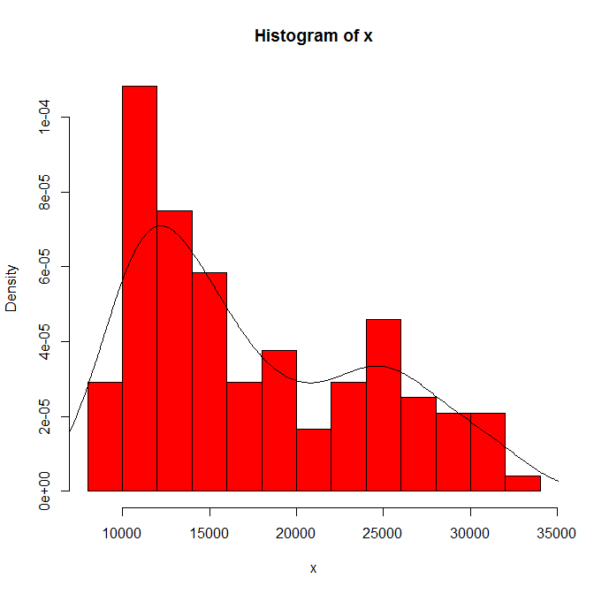
First, let's follow @Glen_b's suggestion and look at your data using twice as many bins:

enter image description here

We still see two modes; if anything, they come through more clearly here. (Note also that the kernel density line should be identical, but appears more spread out due to the larger number of bins.)

Now lets fit a Gaussian finite mixture model:

library(mclust)
x.gmm = Mclust(x)
summary(x.gmm)
# ----------------------------------------------------
# Gaussian finite mixture model fitted by EM algorithm 
# ----------------------------------------------------
#   
# Mclust V (univariate, unequal variance) model with 2 components:
#   
#   log.likelihood   n df       BIC       ICL
#        -1200.874 120  5 -2425.686 -2442.719
# 
# Clustering table:
#  1  2 
# 68 52 

Two normal components optimizes the BIC. For comparison, we can force a one component fit and perform a likelihood ratio test:

x.gmm.1 = Mclust(x, G=1)
logLik(x.gmm.1)
# 'log Lik.' -1226.241 (df=2)
logLik(x.gmm)-logLik(x.gmm.1)
# 'log Lik.' 25.36657 (df=5)
1-pchisq(25.36657, df=3)  # [1] 1.294187e-05

This suggests it is extremely unlikely you would find data as far from unimodal as yours if they came from a single true normal distribution.

Some people don't feel comfortable using a parametric test here (although if the assumptions hold, I don't know of any problem). One very broadly applicable technique is to use the Parametric Bootstrap Cross-fitting Method (I describe the algorithm here). We can try applying it to these data:

x.gmm$parameters
# $mean
# 12346.98 23322.06 
# $variance$sigmasq
# [1]  4514863 24582180
x.gmm.1$parameters
# $mean
# [1] 17520.91
# $variance$sigmasq
# [1] 43989870

set.seed(7809)
B = 10000;    x2.d = vector(length=B);    x1.d = vector(length=B)
for(i in 1:B){
  x2      = c(rnorm(68, mean=12346.98, sd=sqrt( 4514863)), 
              rnorm(52, mean=23322.06, sd=sqrt(24582180)) )
  x1      = rnorm( 120, mean=17520.91, sd=sqrt(43989870))
  x2.d[i] = Mclust(x2, G=2)$loglik - Mclust(x2, G=1)$loglik
  x1.d[i] = Mclust(x1, G=2)$loglik - Mclust(x1, G=1)$loglik
}
x2.d = sort(x2.d);  x1.d = sort(x1.d)
summary(x1.d)
#     Min.  1st Qu.   Median     Mean  3rd Qu.     Max. 
# -0.29070 -0.02124  0.41460  0.88760  1.36700 14.01000 
summary(x2.d)
#   Min. 1st Qu.  Median    Mean 3rd Qu.    Max. 
#  9.006  23.770  27.500  27.760  31.350  53.500 

enter image description here

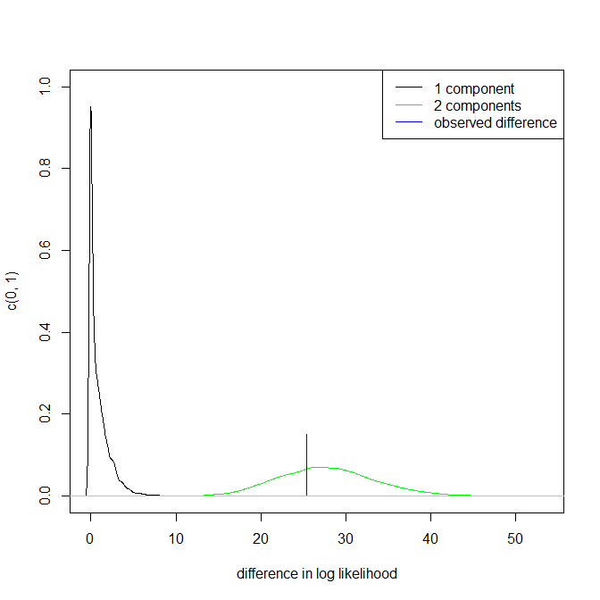
The summary statistics, and the kernel density plots for the sampling distributions show several interesting features. The log likelihood for the single component model is rarely greater than that of the two component fit, even when the true data generating process has only a single component, and when it is greater, the amount is trivial. The idea of comparing models that differ in their ability to fit data is one of the motivations behind the PBCM. The two sampling distributions barely overlap at all; only .35% of x2.d are less than the maximum x1.d value. If you selected a two component model if the difference in log likelihood were >9.7, you would incorrectly select the one component model .01% and the two component model .02% of the time. These are highly discriminable. If, on the other hand, you chose to use the one component model as a null hypothesis, your observed result is sufficiently small as not to show up in the empirical sampling distribution in 10,000 iterations. We can use the rule of 3 (see here) to place an upper bound on the p-value, namely, we estimate your p-value is less than .0003. That is, this is highly significant.

This raises the question of why these results diverge so much from your dip test. (To answer your explicit question, your dip test provides no evidence that there are two real modes.) I honestly don't know the dip test, so it's hard to say; it may be underpowered. However, I think the likely answer is that this approach assumes your data are generated by true normal[s]. A Shapiro-Wilk test for your data is highly significant ($p < .000001$), and it is also highly significant for the optimal Box-Cox transformation of your data (the inverse square root; $p < .001$). However, data are never really normal (cf., this famous quote), and the underlying components, should they exist, aren't guaranteed to be perfectly normal either. If you find it reasonable that your data could come from a positively skewed distribution, rather than a normal, this level of bimodality may well be within the typical range of variation, which is what I suspect the dip test is saying.