added 64 characters in body
Source Link
kjetil b halvorsen
  • 82.8k
  • 32
  • 201
  • 663
  # kernel density estimate for x using Sheather-Jones method to estimate b/w:
density(x, kernel="gaussian", bw="SJ") -> dens.SJ
  # tweak b/w until mode just disappears:
density(x, kernel="gaussian", bw=3160) -> prox.null
  # fill matrix with simulated samples from the proximal null:
x.sim <- matrix(NA, nrow=length(x), ncol=10)
for (i in 1:10){
  x.sim[ ,i] <- rnorm(length(x), sample(x, size=length(x), replace=T), prox.null$bw)
}
  # perform Silverman test without Hall-York calibration:
require(silvermantest)
silverman.test(x, k=1, M=10000, adjust=F)
  # perform Silverman test with Hall-York calibration:
silverman.test(x, k=1, M=10000, adjust=T)
      # kernel density estimate for x using Sheather-Jones 
          # method to estimate b/w:
    density(x, kernel="gaussian", bw="SJ") -> dens.SJ
      # tweak b/w until mode just disappears:
    density(x, kernel="gaussian", bw=3160) -> prox.null
      # fill matrix with simulated samples from the proximal 
      # null:
    x.sim <- matrix(NA, nrow=length(x), ncol=10)
    for (i in 1:10){
      x.sim[ ,i] <- rnorm(length(x), sample(x, size=length(x), 
                          replace=TRUE), prox.null$bw)
    }
      # perform Silverman test without Hall-York calibration:
    require(silvermantest)
    silverman.test(x, k=1, M=10000, adjust=F)
      # perform Silverman test with Hall-York calibration:
    silverman.test(x, k=1, M=10000, adjust=T)

Following up on the ideas in @Nick's answer and comments, you can see how wide the bandwidth needs to be to just flatten out the secondary mode:
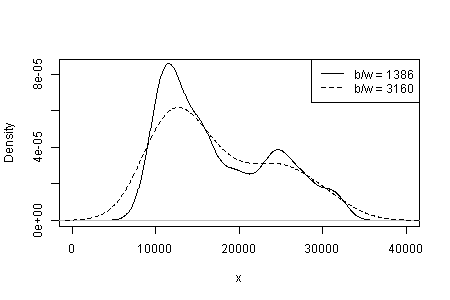
enter image description here

Take this kernel density estimate as the proximal null—the distribution closest to the data yet still consistent with the null hypothesis that it's a sample from a unimodal population—and simulate from it. In the simulated samples the secondary mode doesn't often look so distinct, and you needn't widen the bandwidth as much to flatten it out.

enter image description here

Formalizing this approach leads to the test given in Silverman (1981), "Using kernel density estimates to investigate modality", JRSS B, 43, 1. Schwaiger & Holzmann's silvermantest packagesilvermantest package implements this test, and also the calibration procedure described by Hall & York (2001), "On the calibration of Silverman's test for multimodality", Statistica Sinica, 11, p 515, which adjusts for asymptotic conservatism. Performing the test on your data with a null hypothesis of unimodality results in p-values of 0.08 without calibration and 0.02 with calibration. I'm not familiar enough with the dip test to guess at why it might differ.

R code:

  # kernel density estimate for x using Sheather-Jones method to estimate b/w:
density(x, kernel="gaussian", bw="SJ") -> dens.SJ
  # tweak b/w until mode just disappears:
density(x, kernel="gaussian", bw=3160) -> prox.null
  # fill matrix with simulated samples from the proximal null:
x.sim <- matrix(NA, nrow=length(x), ncol=10)
for (i in 1:10){
  x.sim[ ,i] <- rnorm(length(x), sample(x, size=length(x), replace=T), prox.null$bw)
}
  # perform Silverman test without Hall-York calibration:
require(silvermantest)
silverman.test(x, k=1, M=10000, adjust=F)
  # perform Silverman test with Hall-York calibration:
silverman.test(x, k=1, M=10000, adjust=T)

Following up on the ideas in @Nick's answer and comments, you can see how wide the bandwidth needs to be to just flatten out the secondary mode:

enter image description here

Take this kernel density estimate as the proximal null—the distribution closest to the data yet still consistent with the null hypothesis that it's a sample from a unimodal population—and simulate from it. In the simulated samples the secondary mode doesn't often look so distinct, and you needn't widen the bandwidth as much to flatten it out.

enter image description here

Formalizing this approach leads to the test given in Silverman (1981), "Using kernel density estimates to investigate modality", JRSS B, 43, 1. Schwaiger & Holzmann's silvermantest package implements this test, and also the calibration procedure described by Hall & York (2001), "On the calibration of Silverman's test for multimodality", Statistica Sinica, 11, p 515, which adjusts for asymptotic conservatism. Performing the test on your data with a null hypothesis of unimodality results in p-values of 0.08 without calibration and 0.02 with calibration. I'm not familiar enough with the dip test to guess at why it might differ.

R code:

  # kernel density estimate for x using Sheather-Jones method to estimate b/w:
density(x, kernel="gaussian", bw="SJ") -> dens.SJ
  # tweak b/w until mode just disappears:
density(x, kernel="gaussian", bw=3160) -> prox.null
  # fill matrix with simulated samples from the proximal null:
x.sim <- matrix(NA, nrow=length(x), ncol=10)
for (i in 1:10){
  x.sim[ ,i] <- rnorm(length(x), sample(x, size=length(x), replace=T), prox.null$bw)
}
  # perform Silverman test without Hall-York calibration:
require(silvermantest)
silverman.test(x, k=1, M=10000, adjust=F)
  # perform Silverman test with Hall-York calibration:
silverman.test(x, k=1, M=10000, adjust=T)
light editing & formatting
Source Link
gung - Reinstate Monica
  • 147.5k
  • 89
  • 406
  • 717

Following up on the ideas in @Nick's answer &and comments, you can see how wide the bandwidth needs to be to just flatten out the secondary mode:

enter image description here

Take this kernel density estimate as the proximal null—the distribution closest to the data yet still consistent with the null hypothesis that it's a sample from a unimodal population— &population—and simulate from it. In the simulated samples the secondary mode doesn't often look so distinct, &and you needn't widen the bandwidth as much to flatten it out.
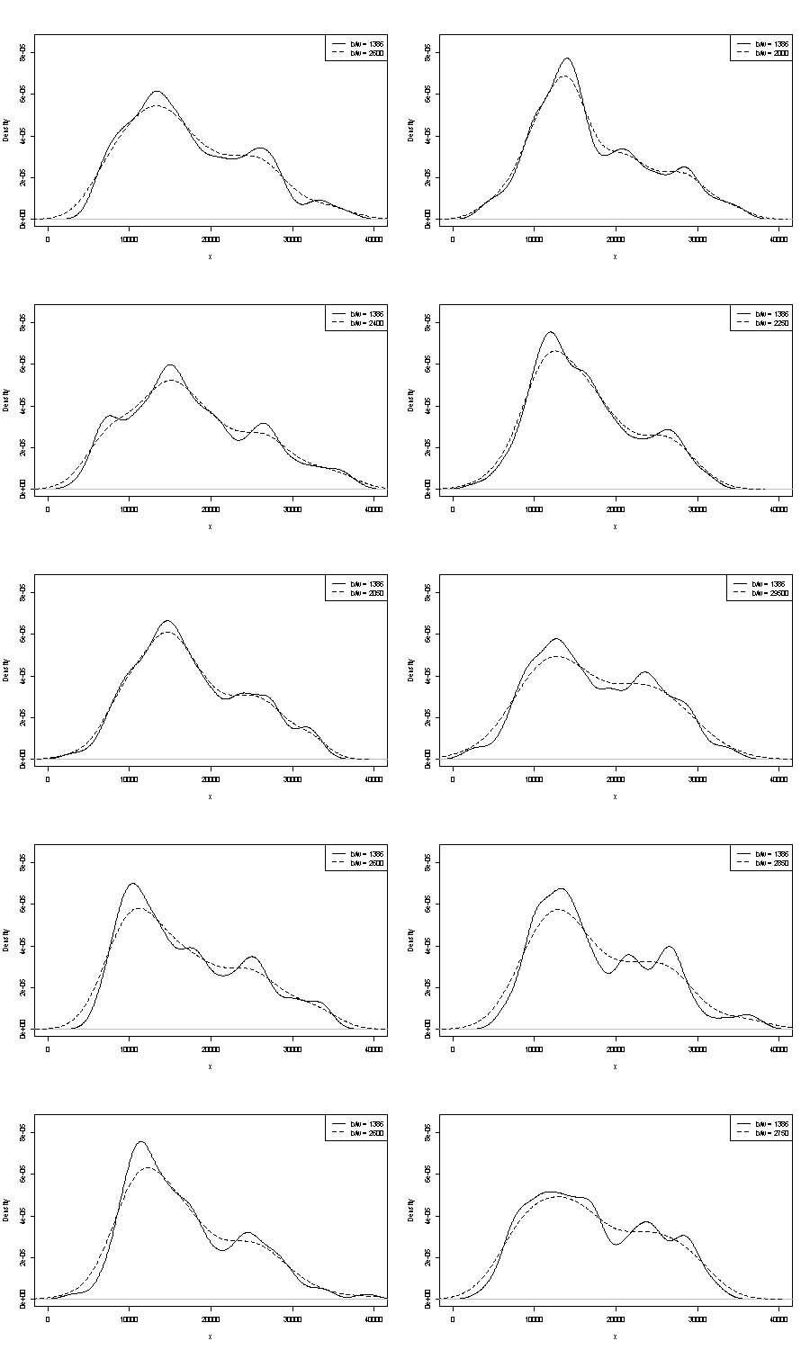
enter image description here

Formalizing this approach leads to the test given in Silverman (1981), "Using kernel density estimates to investigate modality", JRSS B, 43, 1. Schwaiger & Holzmann's silvermantest package implements this test, & alsotheand also the calibration procedure described by Hall & York (2001), "On the calibration of Silverman's test for multimodality", Statistica Sinica, 11, p515p 515, which adjusts for asymptotic conservatism. Performing the test on your data with a null hypothesis of unimodality results in p-values of 0.08 without calibration &and 0.02 with calibration. I'm not familiar enough with the dip test to guess at why it might differ.

R code:

  # kernel density estimate for x using Sheather-Jones method to estimate b/w:
density(x, kernel="gaussian", bw="SJ") -> dens.SJ
  # tweak b/w until mode just disappears:
density(x, kernel="gaussian", bw=3160) -> prox.null
  # fill matrix with simulated samples from the proximal null:
x.sim <- matrix(NA, nrow=length(x), ncol=10)
for (i in 1:10){
  x.sim[ ,i] <- rnorm(length(x), sample(x, size = lengthsize=length(x), replace = Treplace=T), prox.null$bw)
}
  # perform Silverman test without Hall-York calibration:
require(silvermantest)
silverman.test(x, k=1, M=10000, adjust=F)
  # perform Silverman test with Hall-York calibration:
silverman.test(x, k=1, M=10000, adjust=T)

Following up on the ideas in @Nick's answer & comments, you can see how wide the bandwidth needs to be to just flatten out the secondary mode:

enter image description here

Take this kernel density estimate as the proximal null—the distribution closest to the data yet still consistent with the null hypothesis that it's a sample from a unimodal population— & simulate from it. In the simulated samples the secondary mode doesn't often look so distinct, & you needn't widen the bandwidth as much to flatten it out.

enter image description here

Formalizing this approach leads to the test given in Silverman (1981), "Using kernel density estimates to investigate modality", JRSS B, 43, 1. Schwaiger & Holzmann's silvermantest package implements this test, & alsothe calibration procedure described by Hall & York (2001), "On the calibration of Silverman's test for multimodality", Statistica Sinica, 11, p515, which adjusts for asymptotic conservatism. Performing the test on your data with a null hypothesis of unimodality results in p-values of 0.08 without calibration & 0.02 with calibration. I'm not familiar enough with the dip test to guess at why it might differ.

R code:

# kernel density estimate for x using Sheather-Jones method to estimate b/w
density(x, kernel="gaussian", bw="SJ") -> dens.SJ
# tweak b/w until mode just disappears
density(x, kernel="gaussian", bw=3160) -> prox.null
# fill matrix with simulated samples from the proximal null
x.sim <- matrix(NA, nrow=length(x), ncol=10)
for (i in 1:10){
x.sim[ ,i] <- rnorm(length(x), sample(x, size = length(x), replace = T), prox.null$bw)
}
# perform Silverman test without Hall-York calibration
require(silvermantest)
silverman.test(x, k=1, M=10000, adjust=F)
# perform Silverman test with Hall-York calibration
silverman.test(x, k=1, M=10000, adjust=T)

Following up on the ideas in @Nick's answer and comments, you can see how wide the bandwidth needs to be to just flatten out the secondary mode:

enter image description here

Take this kernel density estimate as the proximal null—the distribution closest to the data yet still consistent with the null hypothesis that it's a sample from a unimodal population—and simulate from it. In the simulated samples the secondary mode doesn't often look so distinct, and you needn't widen the bandwidth as much to flatten it out.

enter image description here

Formalizing this approach leads to the test given in Silverman (1981), "Using kernel density estimates to investigate modality", JRSS B, 43, 1. Schwaiger & Holzmann's silvermantest package implements this test, and also the calibration procedure described by Hall & York (2001), "On the calibration of Silverman's test for multimodality", Statistica Sinica, 11, p 515, which adjusts for asymptotic conservatism. Performing the test on your data with a null hypothesis of unimodality results in p-values of 0.08 without calibration and 0.02 with calibration. I'm not familiar enough with the dip test to guess at why it might differ.

R code:

  # kernel density estimate for x using Sheather-Jones method to estimate b/w:
density(x, kernel="gaussian", bw="SJ") -> dens.SJ
  # tweak b/w until mode just disappears:
density(x, kernel="gaussian", bw=3160) -> prox.null
  # fill matrix with simulated samples from the proximal null:
x.sim <- matrix(NA, nrow=length(x), ncol=10)
for (i in 1:10){
  x.sim[ ,i] <- rnorm(length(x), sample(x, size=length(x), replace=T), prox.null$bw)
}
  # perform Silverman test without Hall-York calibration:
require(silvermantest)
silverman.test(x, k=1, M=10000, adjust=F)
  # perform Silverman test with Hall-York calibration:
silverman.test(x, k=1, M=10000, adjust=T)
added 790 characters in body
Source Link
Scortchi
  • 31.6k
  • 9
  • 102
  • 282
Loading
added 486 characters in body
Source Link
Scortchi
  • 31.6k
  • 9
  • 102
  • 282
Loading
Source Link
Scortchi
  • 31.6k
  • 9
  • 102
  • 282
Loading