replaced http://stats.stackexchange.com/ with https://stats.stackexchange.com/
Source Link

To understand interactions in logistic regression, I found this postingthis posting helpful.

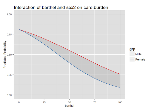
I personally find visual inspection helpful, especially when you have interaction terms in logistic regression. In my sjPlot-package there's a function to plot interaction terms of (generalized) linear (mixed effects) models. You can find some examples in this online-manual. The formula to calculate the interaction is based on what Karen Grace described here and here.

For logistic regressions, the odds ratios are translated into probabilities.

Here's an example from the sample data set with a simple glm:

# load sample data
data(efc)
# create binary response
care.burden <- ifelse(efc$neg_c_7 < median(na.omit(efc$neg_c_7)), 0, 1)
# create data frame for fitted model
mydf <- data.frame(care.burden = as.factor(care.burden),
                   sex = as.factor(efc$c161sex),
                   barthel = as.numeric(efc$barthtot))
# fit model
fit <- glm(care.burden ~ sex * barthel,
           data = mydf,
           family = binomial(link = "logit"),
           x = TRUE)
# plot interaction, increase p-level sensivity
sjp.int(fit,
        legendLabels = get_val_labels(efc$c161sex),
        plevel = 0.1)
enter image description here

To understand interactions in logistic regression, I found this posting helpful.

I personally find visual inspection helpful, especially when you have interaction terms in logistic regression. In my sjPlot-package there's a function to plot interaction terms of (generalized) linear (mixed effects) models. You can find some examples in this online-manual. The formula to calculate the interaction is based on what Karen Grace described here and here.

For logistic regressions, the odds ratios are translated into probabilities.

Here's an example from the sample data set with a simple glm:

# load sample data
data(efc)
# create binary response
care.burden <- ifelse(efc$neg_c_7 < median(na.omit(efc$neg_c_7)), 0, 1)
# create data frame for fitted model
mydf <- data.frame(care.burden = as.factor(care.burden),
                   sex = as.factor(efc$c161sex),
                   barthel = as.numeric(efc$barthtot))
# fit model
fit <- glm(care.burden ~ sex * barthel,
           data = mydf,
           family = binomial(link = "logit"),
           x = TRUE)
# plot interaction, increase p-level sensivity
sjp.int(fit,
        legendLabels = get_val_labels(efc$c161sex),
        plevel = 0.1)

enter image description here

To understand interactions in logistic regression, I found this posting helpful.

I personally find visual inspection helpful, especially when you have interaction terms in logistic regression. In my sjPlot-package there's a function to plot interaction terms of (generalized) linear (mixed effects) models. You can find some examples in this online-manual. The formula to calculate the interaction is based on what Karen Grace described here and here.

For logistic regressions, the odds ratios are translated into probabilities.

Here's an example from the sample data set with a simple glm:

# load sample data
data(efc)
# create binary response
care.burden <- ifelse(efc$neg_c_7 < median(na.omit(efc$neg_c_7)), 0, 1)
# create data frame for fitted model
mydf <- data.frame(care.burden = as.factor(care.burden),
                   sex = as.factor(efc$c161sex),
                   barthel = as.numeric(efc$barthtot))
# fit model
fit <- glm(care.burden ~ sex * barthel,
           data = mydf,
           family = binomial(link = "logit"),
           x = TRUE)
# plot interaction, increase p-level sensivity
sjp.int(fit,
        legendLabels = get_val_labels(efc$c161sex),
        plevel = 0.1)

enter image description here

typo
Source Link
Daniel
  • 1.4k
  • 10
  • 18

To understand interactions in logistic regression, I found this posting helpful.

I personally find visual inspection helpful, especially when you have interaction terms in logistic regression. In my sjPlot-package there's a function to plot interaction terms of (generalized) linear (mixed effects) models. You can find some examples in this online-manual. The formula to calculate the interaction is based on what Karen Grace described here and here.

For logistic regressions, the odds ratios are translated into probabilities.

Here's an example from the sample data set with a simple glm:

# load sample data
data(efc)
# create binary response
care.burden <- ifelse(efc$neg_c_7 < median(na.omit(efc$neg_c_7)), 0, 1)
# create data frame for fitted model
mydf <- data.frame(care.burden = as.factor(care.burden),
                   sex = as.factor(efc$c161sex),
                   barthel = as.numeric(efc$barthtot))
# fit model
fit <- glm(care.burden ~ sex * barthel,
           data = mydf,
           family = binomial(link = "logit"),
           x = TRUE)
# plot interaction, increase p-level sensivity
sjp.int(fit,
        legendLabels = sji.getValueLabelsget_val_labels(efc$c161sex),
        plevel = 0.1)

enter image description here

To understand interactions in logistic regression, I found this posting helpful.

I personally find visual inspection helpful, especially when you have interaction terms in logistic regression. In my sjPlot-package there's a function to plot interaction terms of (generalized) linear (mixed effects) models. You can find some examples in this online-manual. The formula to calculate the interaction is based on what Karen Grace described here and here.

For logistic regressions, the odds ratios are translated into probabilities.

Here's an example from the sample data set with a simple glm:

# load sample data
data(efc)
# create binary response
care.burden <- ifelse(efc$neg_c_7 < median(na.omit(efc$neg_c_7)), 0, 1)
# create data frame for fitted model
mydf <- data.frame(care.burden = as.factor(care.burden),
                   sex = as.factor(efc$c161sex),
                   barthel = as.numeric(efc$barthtot))
# fit model
fit <- glm(care.burden ~ sex * barthel,
           data = mydf,
           family = binomial(link = "logit"),
           x = TRUE)
# plot interaction, increase p-level sensivity
sjp.int(fit,
        legendLabels = sji.getValueLabels(efc$c161sex),
        plevel = 0.1)

enter image description here

To understand interactions in logistic regression, I found this posting helpful.

I personally find visual inspection helpful, especially when you have interaction terms in logistic regression. In my sjPlot-package there's a function to plot interaction terms of (generalized) linear (mixed effects) models. You can find some examples in this online-manual. The formula to calculate the interaction is based on what Karen Grace described here and here.

For logistic regressions, the odds ratios are translated into probabilities.

Here's an example from the sample data set with a simple glm:

# load sample data
data(efc)
# create binary response
care.burden <- ifelse(efc$neg_c_7 < median(na.omit(efc$neg_c_7)), 0, 1)
# create data frame for fitted model
mydf <- data.frame(care.burden = as.factor(care.burden),
                   sex = as.factor(efc$c161sex),
                   barthel = as.numeric(efc$barthtot))
# fit model
fit <- glm(care.burden ~ sex * barthel,
           data = mydf,
           family = binomial(link = "logit"),
           x = TRUE)
# plot interaction, increase p-level sensivity
sjp.int(fit,
        legendLabels = get_val_labels(efc$c161sex),
        plevel = 0.1)

enter image description here

Source Link
Daniel
  • 1.4k
  • 10
  • 18

To understand interactions in logistic regression, I found this posting helpful.

I personally find visual inspection helpful, especially when you have interaction terms in logistic regression. In my sjPlot-package there's a function to plot interaction terms of (generalized) linear (mixed effects) models. You can find some examples in this online-manual. The formula to calculate the interaction is based on what Karen Grace described here and here.

For logistic regressions, the odds ratios are translated into probabilities.

Here's an example from the sample data set with a simple glm:

# load sample data
data(efc)
# create binary response
care.burden <- ifelse(efc$neg_c_7 < median(na.omit(efc$neg_c_7)), 0, 1)
# create data frame for fitted model
mydf <- data.frame(care.burden = as.factor(care.burden),
                   sex = as.factor(efc$c161sex),
                   barthel = as.numeric(efc$barthtot))
# fit model
fit <- glm(care.burden ~ sex * barthel,
           data = mydf,
           family = binomial(link = "logit"),
           x = TRUE)
# plot interaction, increase p-level sensivity
sjp.int(fit,
        legendLabels = sji.getValueLabels(efc$c161sex),
        plevel = 0.1)

enter image description here