edited body
Source Link
Richard Hardy
  • 69.5k
  • 13
  • 126
  • 278

Recently I tried to fit some points which (from the plot) seems linearly distributed. The fit result (in R) is:

Residuals:
    Min      1Q  Median      3Q     Max 
-112223   -2532    2021    3698   83241 

Coefficients:
              Estimate Std. Error t value Pr(>|t|)    
(Intercept) -6.623e+03  7.136e+02  -9.282   <2e-16 ***
population   5.946e-02  4.278e-04 138.986   <2e-16 ***
---
Signif. codes:  0 ‘***’ 0.001 ‘**’ 0.01 ‘*’ 0.05 ‘.’ 0.1 ‘ ’ 1

Residual standard error: 12780 on 379 degrees of freedom
Multiple R-squared:  0.9808,    Adjusted R-squared:  0.9807 
F-statistic: 1.932e+04 on 1 and 379 DF,  p-value: < 2.2e-16

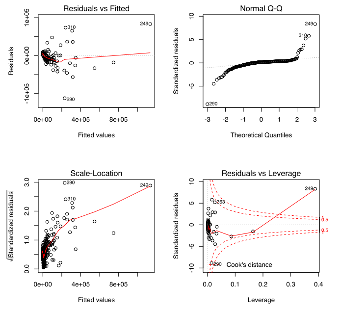
With $R^2$ 0.98. Nice! BUT I checked the OLS assumptions and from the graph I have heteroscedasticity (top-left and bottom-left graph) and I have no normality of errors (top-right graph).

enter image description here

So I transformed the dependantdependent and independantindependent variables with log transformation. I now have a model which meet all the assumptions but it is more complicated (exponential fit?) and with lower $R^2$: 0.96.

Residuals:
     Min       1Q   Median       3Q      Max 
-0.37058 -0.06061 -0.00701  0.05532  0.44428 

Coefficients:
               Estimate Std. Error t value Pr(>|t|)    
(Intercept)    -2.08467    0.06153  -33.88   <2e-16 ***
log_population  1.12146    0.01120  100.12   <2e-16 ***
---
Signif. codes:  0 ‘***’ 0.001 ‘**’ 0.01 ‘*’ 0.05 ‘.’ 0.1 ‘ ’ 1

Residual standard error: 0.101 on 379 degrees of freedom
Multiple R-squared:  0.9636,    Adjusted R-squared:  0.9635 
F-statistic: 1.002e+04 on 1 and 379 DF,  p-value: < 2.2e-16

Which is the best? Is the first model wrong, and why?

Recently I tried to fit some points which (from the plot) seems linearly distributed. The fit result (in R) is:

Residuals:
    Min      1Q  Median      3Q     Max 
-112223   -2532    2021    3698   83241 

Coefficients:
              Estimate Std. Error t value Pr(>|t|)    
(Intercept) -6.623e+03  7.136e+02  -9.282   <2e-16 ***
population   5.946e-02  4.278e-04 138.986   <2e-16 ***
---
Signif. codes:  0 ‘***’ 0.001 ‘**’ 0.01 ‘*’ 0.05 ‘.’ 0.1 ‘ ’ 1

Residual standard error: 12780 on 379 degrees of freedom
Multiple R-squared:  0.9808,    Adjusted R-squared:  0.9807 
F-statistic: 1.932e+04 on 1 and 379 DF,  p-value: < 2.2e-16

With $R^2$ 0.98. Nice! BUT I checked the OLS assumptions and from the graph I have heteroscedasticity (top-left and bottom-left graph) and I have no normality of errors (top-right graph).

enter image description here

So I transformed the dependant and independant variables with log transformation. I now have a model which meet all the assumptions but it is more complicated (exponential fit?) and with lower $R^2$: 0.96.

Residuals:
     Min       1Q   Median       3Q      Max 
-0.37058 -0.06061 -0.00701  0.05532  0.44428 

Coefficients:
               Estimate Std. Error t value Pr(>|t|)    
(Intercept)    -2.08467    0.06153  -33.88   <2e-16 ***
log_population  1.12146    0.01120  100.12   <2e-16 ***
---
Signif. codes:  0 ‘***’ 0.001 ‘**’ 0.01 ‘*’ 0.05 ‘.’ 0.1 ‘ ’ 1

Residual standard error: 0.101 on 379 degrees of freedom
Multiple R-squared:  0.9636,    Adjusted R-squared:  0.9635 
F-statistic: 1.002e+04 on 1 and 379 DF,  p-value: < 2.2e-16

Which is the best? Is the first model wrong, and why?
Recently I tried to fit some points which (from the plot) seems linearly distributed. The fit result (in R) is:

Residuals:
    Min      1Q  Median      3Q     Max 
-112223   -2532    2021    3698   83241 

Coefficients:
              Estimate Std. Error t value Pr(>|t|)    
(Intercept) -6.623e+03  7.136e+02  -9.282   <2e-16 ***
population   5.946e-02  4.278e-04 138.986   <2e-16 ***
---
Signif. codes:  0 ‘***’ 0.001 ‘**’ 0.01 ‘*’ 0.05 ‘.’ 0.1 ‘ ’ 1

Residual standard error: 12780 on 379 degrees of freedom
Multiple R-squared:  0.9808,    Adjusted R-squared:  0.9807 
F-statistic: 1.932e+04 on 1 and 379 DF,  p-value: < 2.2e-16

With $R^2$ 0.98. Nice! BUT I checked the OLS assumptions and from the graph I have heteroscedasticity (top-left and bottom-left graph) and I have no normality of errors (top-right graph).

enter image description here

So I transformed the dependent and independent variables with log transformation. I now have a model which meet all the assumptions but it is more complicated (exponential fit?) and with lower $R^2$: 0.96.

Residuals:
     Min       1Q   Median       3Q      Max 
-0.37058 -0.06061 -0.00701  0.05532  0.44428 

Coefficients:
               Estimate Std. Error t value Pr(>|t|)    
(Intercept)    -2.08467    0.06153  -33.88   <2e-16 ***
log_population  1.12146    0.01120  100.12   <2e-16 ***
---
Signif. codes:  0 ‘***’ 0.001 ‘**’ 0.01 ‘*’ 0.05 ‘.’ 0.1 ‘ ’ 1

Residual standard error: 0.101 on 379 degrees of freedom
Multiple R-squared:  0.9636,    Adjusted R-squared:  0.9635 
F-statistic: 1.002e+04 on 1 and 379 DF,  p-value: < 2.2e-16

Which is the best? Is the first model wrong, and why?

added 4 characters in body; edited title
Source Link
Tim
  • 141.2k
  • 26
  • 270
  • 512

High R^2$R^2$ on Ordinary least squares model with violated assumptions. Is it good?

Recently I tried to fit some points which (from the plot) seems linearly distributed. The fit result (in R) is:

Residuals:
    Min      1Q  Median      3Q     Max 
-112223   -2532    2021    3698   83241 

Coefficients:
              Estimate Std. Error t value Pr(>|t|)    
(Intercept) -6.623e+03  7.136e+02  -9.282   <2e-16 ***
population   5.946e-02  4.278e-04 138.986   <2e-16 ***
---
Signif. codes:  0 ‘***’ 0.001 ‘**’ 0.01 ‘*’ 0.05 ‘.’ 0.1 ‘ ’ 1

Residual standard error: 12780 on 379 degrees of freedom
Multiple R-squared:  0.9808,    Adjusted R-squared:  0.9807 
F-statistic: 1.932e+04 on 1 and 379 DF,  p-value: < 2.2e-16

With R^2$R^2$ 0.98. Nice! BUT I checked the OLS assumptions and from the graph I have heteroscedasticity (top-left and bottom-left graph) and I have no normality of errors (top-right graph).

enter image description here

So I transformed the dependant and independant variables with log transformation. I now have a model which meet all the assumptions but it is more complicated (exponential fit?) and with lower R^2$R^2$: 0.96.

Residuals:
     Min       1Q   Median       3Q      Max 
-0.37058 -0.06061 -0.00701  0.05532  0.44428 

Coefficients:
               Estimate Std. Error t value Pr(>|t|)    
(Intercept)    -2.08467    0.06153  -33.88   <2e-16 ***
log_population  1.12146    0.01120  100.12   <2e-16 ***
---
Signif. codes:  0 ‘***’ 0.001 ‘**’ 0.01 ‘*’ 0.05 ‘.’ 0.1 ‘ ’ 1

Residual standard error: 0.101 on 379 degrees of freedom
Multiple R-squared:  0.9636,    Adjusted R-squared:  0.9635 
F-statistic: 1.002e+04 on 1 and 379 DF,  p-value: < 2.2e-16

Which is the best? Is the first model wrong, and why?

High R^2 on Ordinary least squares model with violated assumptions. Is it good?

Recently I tried to fit some points which (from the plot) seems linearly distributed. The fit result (in R) is:

Residuals:
    Min      1Q  Median      3Q     Max 
-112223   -2532    2021    3698   83241 

Coefficients:
              Estimate Std. Error t value Pr(>|t|)    
(Intercept) -6.623e+03  7.136e+02  -9.282   <2e-16 ***
population   5.946e-02  4.278e-04 138.986   <2e-16 ***
---
Signif. codes:  0 ‘***’ 0.001 ‘**’ 0.01 ‘*’ 0.05 ‘.’ 0.1 ‘ ’ 1

Residual standard error: 12780 on 379 degrees of freedom
Multiple R-squared:  0.9808,    Adjusted R-squared:  0.9807 
F-statistic: 1.932e+04 on 1 and 379 DF,  p-value: < 2.2e-16

With R^2 0.98. Nice! BUT I checked the OLS assumptions and from the graph I have heteroscedasticity (top-left and bottom-left graph) and I have no normality of errors (top-right graph).

enter image description here

So I transformed the dependant and independant variables with log transformation. I now have a model which meet all the assumptions but it is more complicated (exponential fit?) and with lower R^2: 0.96.

Residuals:
     Min       1Q   Median       3Q      Max 
-0.37058 -0.06061 -0.00701  0.05532  0.44428 

Coefficients:
               Estimate Std. Error t value Pr(>|t|)    
(Intercept)    -2.08467    0.06153  -33.88   <2e-16 ***
log_population  1.12146    0.01120  100.12   <2e-16 ***
---
Signif. codes:  0 ‘***’ 0.001 ‘**’ 0.01 ‘*’ 0.05 ‘.’ 0.1 ‘ ’ 1

Residual standard error: 0.101 on 379 degrees of freedom
Multiple R-squared:  0.9636,    Adjusted R-squared:  0.9635 
F-statistic: 1.002e+04 on 1 and 379 DF,  p-value: < 2.2e-16

Which is the best? Is the first model wrong, and why?

High $R^2$ on Ordinary least squares model with violated assumptions. Is it good?

Recently I tried to fit some points which (from the plot) seems linearly distributed. The fit result (in R) is:

Residuals:
    Min      1Q  Median      3Q     Max 
-112223   -2532    2021    3698   83241 

Coefficients:
              Estimate Std. Error t value Pr(>|t|)    
(Intercept) -6.623e+03  7.136e+02  -9.282   <2e-16 ***
population   5.946e-02  4.278e-04 138.986   <2e-16 ***
---
Signif. codes:  0 ‘***’ 0.001 ‘**’ 0.01 ‘*’ 0.05 ‘.’ 0.1 ‘ ’ 1

Residual standard error: 12780 on 379 degrees of freedom
Multiple R-squared:  0.9808,    Adjusted R-squared:  0.9807 
F-statistic: 1.932e+04 on 1 and 379 DF,  p-value: < 2.2e-16

With $R^2$ 0.98. Nice! BUT I checked the OLS assumptions and from the graph I have heteroscedasticity (top-left and bottom-left graph) and I have no normality of errors (top-right graph).

enter image description here

So I transformed the dependant and independant variables with log transformation. I now have a model which meet all the assumptions but it is more complicated (exponential fit?) and with lower $R^2$: 0.96.

Residuals:
     Min       1Q   Median       3Q      Max 
-0.37058 -0.06061 -0.00701  0.05532  0.44428 

Coefficients:
               Estimate Std. Error t value Pr(>|t|)    
(Intercept)    -2.08467    0.06153  -33.88   <2e-16 ***
log_population  1.12146    0.01120  100.12   <2e-16 ***
---
Signif. codes:  0 ‘***’ 0.001 ‘**’ 0.01 ‘*’ 0.05 ‘.’ 0.1 ‘ ’ 1

Residual standard error: 0.101 on 379 degrees of freedom
Multiple R-squared:  0.9636,    Adjusted R-squared:  0.9635 
F-statistic: 1.002e+04 on 1 and 379 DF,  p-value: < 2.2e-16

Which is the best? Is the first model wrong, and why?

Source Link
marcodena
  • 647
  • 1
  • 6
  • 13

High R^2 on Ordinary least squares model with violated assumptions. Is it good?

Recently I tried to fit some points which (from the plot) seems linearly distributed. The fit result (in R) is:

Residuals:
    Min      1Q  Median      3Q     Max 
-112223   -2532    2021    3698   83241 

Coefficients:
              Estimate Std. Error t value Pr(>|t|)    
(Intercept) -6.623e+03  7.136e+02  -9.282   <2e-16 ***
population   5.946e-02  4.278e-04 138.986   <2e-16 ***
---
Signif. codes:  0 ‘***’ 0.001 ‘**’ 0.01 ‘*’ 0.05 ‘.’ 0.1 ‘ ’ 1

Residual standard error: 12780 on 379 degrees of freedom
Multiple R-squared:  0.9808,    Adjusted R-squared:  0.9807 
F-statistic: 1.932e+04 on 1 and 379 DF,  p-value: < 2.2e-16

With R^2 0.98. Nice! BUT I checked the OLS assumptions and from the graph I have heteroscedasticity (top-left and bottom-left graph) and I have no normality of errors (top-right graph).

enter image description here

So I transformed the dependant and independant variables with log transformation. I now have a model which meet all the assumptions but it is more complicated (exponential fit?) and with lower R^2: 0.96.

Residuals:
     Min       1Q   Median       3Q      Max 
-0.37058 -0.06061 -0.00701  0.05532  0.44428 

Coefficients:
               Estimate Std. Error t value Pr(>|t|)    
(Intercept)    -2.08467    0.06153  -33.88   <2e-16 ***
log_population  1.12146    0.01120  100.12   <2e-16 ***
---
Signif. codes:  0 ‘***’ 0.001 ‘**’ 0.01 ‘*’ 0.05 ‘.’ 0.1 ‘ ’ 1

Residual standard error: 0.101 on 379 degrees of freedom
Multiple R-squared:  0.9636,    Adjusted R-squared:  0.9635 
F-statistic: 1.002e+04 on 1 and 379 DF,  p-value: < 2.2e-16

Which is the best? Is the first model wrong, and why?