In order to compare the behavior of the different splitting formulas, let's consider a simple example:

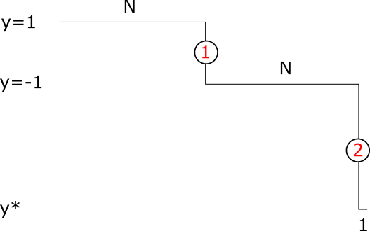
We have $N$ predictors with value $y=1$ in the left, $N$ predictors with value $y=-1$ in the right, and a single point at the right boundary with value $y^\ast$.

When $N$ is large, say $N=100$, I would want the split to be made at the point marked by the red (1).

Let's calculate how low $y^\ast$ might get until the split occurs at (2) -- for which we use the criterium the OP posted in the question, that is the sum of squares (SS) instead of the variance:

Split at (1):

• Mean left: $1$, SS Left: $0$

• Mean right: $\mu_r = (y^\ast - N)/(N+1)$, SS right: $N(-1 - \mu_r)^2 + (y^\ast - \mu_r)^2$

Split at (2):

• Mean left: $0$, SS Left: $2N$

• Mean right: $y^\ast$, SS right: $0$

Setting equal the two sum of squares (SS), Wolfram Alpha gives as solution

$$y^\ast = -1 - \sqrt{2N} \ \underbrace{\sqrt{\frac{(N+1)^2}{(N^2+1)}}}_{\approx 1} \ \approx \ -1 - \sqrt{2N}$$

That means, for a value above this $y^\ast$, the split is made at (1), below $y^\ast$ the split is made at (2).

Now, doing the same for the version where the splitting formula is divided by the number of data points inside the respective region, the result is

$$y^\ast = -1 - \sqrt{\frac{(N+1)^2}{(N^2+1)}}$$

That is, the factor $\sqrt{2N}$ is missing. The split is made at (2) if the value at the boundary is slightly lower than $-1$.

Conclusion: The splitting formula without division of the particle number leads to the imo more intuitive behaviour that the split is done at point (1) in the middle.

This is reasonable, as without the factors the absolute quantities matter. With the normalization by the sample size, one considers average quantities by which -- as seen above -- small regions become similar weight to very large regions.

Summarizing, I would prefer the splitting criterium as the OP gave it in his question.

In order to compare the behavior of the different splitting formulas, let's consider a simple example:

We have $N$ predictors with value $y=1$ in the left, $N$ predictors with value $y=-1$ in the right, and a single point at the right boundary with value $y^\ast$.

There are two reasonable split points in this scenario, first the point (1) in the middle, and the point (2) at the right boundary.

When $N$ is large, say $N=100$, I would prefer the split to be made at the point marked by the red (1). Only if the value of $y^\ast$ becomes very low, I would find a split at (2) reasonable.

So, let's calculate how the split position changes in dependence of the value of $y^\ast$: For which $y^\ast$ is the split made at (1), or how low $y^\ast$ might get until the split occurs at (2).

For the calculations we first use the criterium the OP posted in the question, which involves the sum of squares (SS):

Split at (1):

• Mean left: $1$, SS Left: $0$

• Mean right: $\mu_r = (y^\ast - N)/(N+1)$, SS right: $N(-1 - \mu_r)^2 + (y^\ast - \mu_r)^2$

Split at (2):

• Mean left: $0$, SS Left: $2N$

• Mean right: $y^\ast$, SS right: $0$

Thus, we get a split at point (1) if

$$N(-1 - \mu_r)^2 + (y^\ast - \mu_r)^2 \leq 2N$$

Inserting $\mu_r$ and setting equal the two sum of squares (SS), Wolfram Alpha gives as solution

$$y_{SS}^\ast = -1 - \sqrt{2N} \ \underbrace{\sqrt{\frac{(N+1)^2}{(N^2+1)}}}_{\approx 1} \ \approx \ -1 - \sqrt{2N}$$

That means, for a value $y$ above $y_{SS}^\ast$, the split is made at (1), below $y_{SS}^\ast$ the split is made at (2). One sees that for large $N$ the split is preferred in the middle.

Now, doing the same for the version of the splitting formula which includes the variance, the result is

$$y_{VAR}^\ast = -1 - \sqrt{\frac{(N+1)^2}{(N^2+1)}} \ \approx \ 1$$

That is, the factor $\sqrt{2N}$ is missing. With this, the split is made at (2) if the value at the boundary is slightly lower than $-1$, regardless of the number of datapoints $N$.

Conclusion: The splitting formula using the sum of squares (SS) leads to the more intuitive behaviour that the split is preferred at point (1) in the middle.

Instead, the formula with the variance does not consider the number of particles in the respective regions, as the SS value is divided by the number of data points. As seen above, it easily prefers a split where only one data point is separated to a balanced split where the region is halfed.

Summarizing, I would prefer the splitting criterium containing the sum-of-squares to the splitting criterium containing the variance.

Let's consider an example:

We have $N$ predictors with value $y=1$ in the left, $N$ predictors with value $y=-1$ in the right, and a single point at the right boundary with value $y^\ast$.

When $N$ is large, say $N=100$, I would want the split to be made at the point marked by the red (1).

Let's calculate how low $y^\ast$ might get until the split occurs at (2) -- where we use the criterium the OP posted in the question:

Split at (1):

• Mean left: $1$, Var Left: $0$

• Mean right: $\mu_r = (y^\ast - N)/(N+1)$, Var right: $N(-1 - \mu_r)^2 + (y^\ast - \mu_r)^2$

Split at (2):

• Mean left: $0$, Var Left: $2N$

• Mean right: $y^\ast$, Var right: $0$

Setting equal the two variances, Wolfram Alpha gives as solution

$$y^\ast = -1 - \sqrt{2N} \ \underbrace{\sqrt{\frac{(N+1)^2}{(N^2+1)}}}_{\approx 1} \ \approx \ -1 - \sqrt{2N}$$

That means, for a value above this $y^\ast$, the split is made at (1), below $y^\ast$ the split is made at (2).

Now, doing the same for the version where the splitting formula is divided by the number of data points inside the respective region, the result is

$$y^\ast = -1 - \sqrt{\frac{(N+1)^2}{(N^2+1)}}$$

That is, the factor $\sqrt{2N}$ is missing. The split is made at (2) if the value at the boundary is slightly lower than $-1$.

Conclusion: The splitting formula without division of the particle number leads to the imo more intuitive behaviour that the split is done at point (1) in the middle.

This is reasonable, as without the factors the absolute quantities matter. With the normalization by the sample size, one considers average quantities by which -- as seen above -- small regions become similar weight to very large regions.

Summarizing, I would prefer the splitting criterium as the OP gave it in his question.

In order to compare the behavior of the different splitting formulas, let's consider a simple example:

We have $N$ predictors with value $y=1$ in the left, $N$ predictors with value $y=-1$ in the right, and a single point at the right boundary with value $y^\ast$.

When $N$ is large, say $N=100$, I would want the split to be made at the point marked by the red (1).

Let's calculate how low $y^\ast$ might get until the split occurs at (2) -- for which we use the criterium the OP posted in the question, that is the sum of squares (SS) instead of the variance:

Split at (1):

• Mean left: $1$, SS Left: $0$

• Mean right: $\mu_r = (y^\ast - N)/(N+1)$, SS right: $N(-1 - \mu_r)^2 + (y^\ast - \mu_r)^2$

Split at (2):

• Mean left: $0$, SS Left: $2N$

• Mean right: $y^\ast$, SS right: $0$

Setting equal the two sum of squares (SS), Wolfram Alpha gives as solution

$$y^\ast = -1 - \sqrt{2N} \ \underbrace{\sqrt{\frac{(N+1)^2}{(N^2+1)}}}_{\approx 1} \ \approx \ -1 - \sqrt{2N}$$

That means, for a value above this $y^\ast$, the split is made at (1), below $y^\ast$ the split is made at (2).

Now, doing the same for the version where the splitting formula is divided by the number of data points inside the respective region, the result is

$$y^\ast = -1 - \sqrt{\frac{(N+1)^2}{(N^2+1)}}$$

That is, the factor $\sqrt{2N}$ is missing. The split is made at (2) if the value at the boundary is slightly lower than $-1$.

Conclusion: The splitting formula without division of the particle number leads to the imo more intuitive behaviour that the split is done at point (1) in the middle.

This is reasonable, as without the factors the absolute quantities matter. With the normalization by the sample size, one considers average quantities by which -- as seen above -- small regions become similar weight to very large regions.

Summarizing, I would prefer the splitting criterium as the OP gave it in his question.