MASS, the book (4th edition, page 110) advicesadvises against trying to estimate $\nu$, the degrees of freedom parameter in the t distribution$t$-distribution with maximum likelihood (with some literature references: Lange et al. (1989), "Robust statistical modeling Using the t distribution", JASA, 84, 408, and Fernandez & Steel (1999), "Multivariate Student-t regression models: Pitfalls and inference", Biometrika, 86, 1).

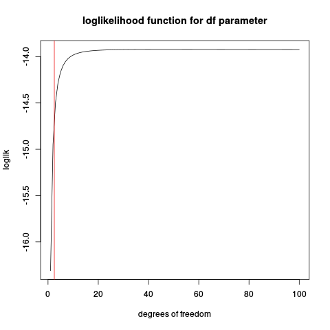
The reason is that the likelihood function for $\nu$ based on the t density function, may be unbounded! and will in those cases not give a well defined maximum. LetLet us seelook at an artificial example where location and scale is known (as the standard $t$-distribution) and only the degrees of freedom is unknown. BelowBelow is some R code, simulating some data, defining the loglikelihoodlog-likelihood function and plotting it:

set.seed(1234)
n <- 10
x <- rt(n,  df=2.5)

make_loglik  <-  function(x)
    Vectorize( function(nu) sum(dt(x, df=nu,  log=TRUE)) )

loglik  <-  make_loglik(x)
plot(loglik,  from=1,  to=100,  main="loglikelihood function for df     parameter", xlab="degrees of freedom")
abline(v=2.5,  col="red2")

enter image description here

If you play around with this code, you can find some cases where there is a well-defined maximum, especially withwhen the sample size $n$ is large. But is the maximum likelihood estimator then any good?

Let us try some simulations:

t_nu_mle  <-  function(x) {
    loglik  <-  make_loglik(x)
    res  <-  optimize(loglik, interval=c(0.01, 200), maximum=TRUE)$maximum
    res   
}

nus  <-  replicate(1000, {x <- rt(10, df=2.5)
    t_nu_mle(x) }, simplify=TRUE)

> mean(nus)
[1] 45.20767
> sd(nus)
[1] 78.77813

Showing the estimation is very unstable (looking at the histogram, a sizeablesizable portion of the estimated values is at the upper limit given to optimize of 200).

Repeating with a larger sample size:

nus  <-  replicate(1000, {x <- rt(50, df=2.5)
    t_nu_mle(x) }, simplify=TRUE)
> mean(nus)
[1] 4.342724
> sd(nus)
[1] 14.40137

which is much better, but the mean is stilstill way above the true value of 2.5.

Then remember that this is a simplified version of the real problem whenwhere location and scale parameters also have to be estimated.

If the reason of using the $t$-distribution is to "robustify", then estimating $\nu$ from the data well may well destroy the robustness.

MASS, the book (4th edition, page 110) advices against trying to estimate $\nu$, the degrees of freedom parameter in the t distribution with maximum likelihood (with some literature references: Lange et al. (1989), "Robust statistical modeling Using the t distribution", JASA, 84, 408, and Fernandez & Steel (1999), "Multivariate Student-t regression models: Pitfalls and inference", Biometrika, 86, 1).

The reason is that the likelihood function for $\nu$ based on the t density function, may be unbounded! and will in those cases not give a well defined maximum. Let us see at an artificial example where location and scale is known (as the standard $t$-distribution) and only the degrees of freedom is unknown. Below is some R code, simulating some data, defining the loglikelihood function and plotting it:

set.seed(1234)
n <- 10
x <- rt(n,  df=2.5)

make_loglik  <-  function(x)
    Vectorize( function(nu) sum(dt(x, df=nu,  log=TRUE)) )

loglik  <-  make_loglik(x)
plot(loglik,  from=1,  to=100,  main="loglikelihood function for df     parameter", xlab="degrees of freedom")
abline(v=2.5,  col="red2")

enter image description here

If you play around with this code, you can find some cases where there is a well-defined maximum, especially with the sample size $n$ large. But is the maximum likelihood estimator then any good?

Let us try some simulations:

t_nu_mle  <-  function(x) {
    loglik  <-  make_loglik(x)
    res  <-  optimize(loglik, interval=c(0.01, 200), maximum=TRUE)$maximum
    res   
}

nus  <-  replicate(1000, {x <- rt(10, df=2.5)
    t_nu_mle(x) }, simplify=TRUE)

> mean(nus)
[1] 45.20767
> sd(nus)
[1] 78.77813

Showing the estimation is very unstable (looking at the histogram, a sizeable portion of the estimated values is at the upper limit given to optimize of 200).

Repeating with a larger sample size:

nus  <-  replicate(1000, {x <- rt(50, df=2.5)
    t_nu_mle(x) }, simplify=TRUE)
> mean(nus)
[1] 4.342724
> sd(nus)
[1] 14.40137

which is much better, but the mean is stil way above the true value of 2.5.

Then remember that this is a simplified version of the real problem when location and scale parameters also have to be estimated.

If the reason of using the $t$-distribution is to "robustify", then estimating $\nu$ from the data well may destroy the robustness.

MASS, the book (4th edition, page 110) advises against trying to estimate $\nu$, the degrees of freedom parameter in the $t$-distribution with maximum likelihood (with some literature references: Lange et al. (1989), "Robust statistical modeling Using the t distribution", JASA, 84, 408, and Fernandez & Steel (1999), "Multivariate Student-t regression models: Pitfalls and inference", Biometrika, 86, 1).

The reason is that the likelihood function for $\nu$ based on the t density function, may be unbounded and will in those cases not give a well defined maximum. Let us look at an artificial example where location and scale is known (as the standard $t$-distribution) and only the degrees of freedom is unknown. Below is some R code, simulating some data, defining the log-likelihood function and plotting it:

set.seed(1234)
n <- 10
x <- rt(n,  df=2.5)

make_loglik  <-  function(x)
    Vectorize( function(nu) sum(dt(x, df=nu,  log=TRUE)) )

loglik  <-  make_loglik(x)
plot(loglik,  from=1,  to=100,  main="loglikelihood function for df     parameter", xlab="degrees of freedom")
abline(v=2.5,  col="red2")

enter image description here

If you play around with this code, you can find some cases where there is a well-defined maximum, especially when the sample size $n$ is large. But is the maximum likelihood estimator then any good?

Let us try some simulations:

t_nu_mle  <-  function(x) {
    loglik  <-  make_loglik(x)
    res  <-  optimize(loglik, interval=c(0.01, 200), maximum=TRUE)$maximum
    res   
}

nus  <-  replicate(1000, {x <- rt(10, df=2.5)
    t_nu_mle(x) }, simplify=TRUE)

> mean(nus)
[1] 45.20767
> sd(nus)
[1] 78.77813

Showing the estimation is very unstable (looking at the histogram, a sizable portion of the estimated values is at the upper limit given to optimize of 200).

Repeating with a larger sample size:

nus  <-  replicate(1000, {x <- rt(50, df=2.5)
    t_nu_mle(x) }, simplify=TRUE)
> mean(nus)
[1] 4.342724
> sd(nus)
[1] 14.40137

which is much better, but the mean is still way above the true value of 2.5.

Then remember that this is a simplified version of the real problem where location and scale parameters also have to be estimated.

If the reason of using the $t$-distribution is to "robustify", then estimating $\nu$ from the data may well destroy the robustness.

added references
Source Link
Scortchi
  • 31.6k
  • 9
  • 102
  • 282

MASS, the book (4th edition, page 110) advices against trying to estimate $\nu$, the degrees of freedom parameter in the t distribution with maximum likelihood (with some literature references I will add in here when I have the book with me: Lange et al. (1989), "Robust statistical modeling Using the t distribution", JASA, 84, 408, and Fernandez & Steel (1999), "Multivariate Student-t regression models: Pitfalls and inference", Biometrika, 86, 1).

The reason is that the likelihood function for $\nu$ based on the t density function, may be unbounded! and will in those cases not give a well defined maximum. Let us see at an artificial example where location and scale is known (as the standard $t$-distribution) and only the degrees of freedom is unknown. Below is some R code, simulating some data, defining the loglikelihood function and plotting it:

set.seed(1234)
n <- 10
x <- rt(n,  df=2.5)

make_loglik  <-  function(x)
    Vectorize( function(nu) sum(dt(x, df=nu,  log=TRUE)) )

loglik  <-  make_loglik(x)
plot(loglik,  from=1,  to=100,  main="loglikelihood function for df     parameter", xlab="degrees of freedom")
abline(v=2.5,  col="red2")

enter image description here

If you play around with this code, you can find some cases where there is a well-defined maximum, especially with the sample size $n$ large. But is the maximum likelihood estimator then any good?

Let us try some simulations:

t_nu_mle  <-  function(x) {
    loglik  <-  make_loglik(x)
    res  <-  optimize(loglik, interval=c(0.01, 200), maximum=TRUE)$maximum
    res   
}

nus  <-  replicate(1000, {x <- rt(10, df=2.5)
    t_nu_mle(x) }, simplify=TRUE)

> mean(nus)
[1] 45.20767
> sd(nus)
[1] 78.77813

Showing the estimation is very unstable (looking at the histogram, a sizeable portion of the estimated values is at the upper limit given to optimize of 200).

Repeating with a larger sample size:

nus  <-  replicate(1000, {x <- rt(50, df=2.5)
    t_nu_mle(x) }, simplify=TRUE)
> mean(nus)
[1] 4.342724
> sd(nus)
[1] 14.40137

which is much better, but the mean is stil way above the true value of 2.5.

Then remember that this is a simplified version of the real problem when location and scale parameters also have to be estimated.

If the reason of using the $t$-distribution is to "robustify", then estimating $\nu$ from the data well may destroy the robustness.

MASS, the book (4th edition, page 110) advices against trying to estimate $\nu$, the degrees of freedom parameter in the t distribution with maximum likelihood (with some literature references I will add in here when I have the book with me).

The reason is that the likelihood function for $\nu$ based on the t density function, may be unbounded! and will in those cases not give a well defined maximum. Let us see at an artificial example where location and scale is known (as the standard $t$-distribution) and only the degrees of freedom is unknown. Below is some R code, simulating some data, defining the loglikelihood function and plotting it:

set.seed(1234)
n <- 10
x <- rt(n,  df=2.5)

make_loglik  <-  function(x)
    Vectorize( function(nu) sum(dt(x, df=nu,  log=TRUE)) )

loglik  <-  make_loglik(x)
plot(loglik,  from=1,  to=100,  main="loglikelihood function for df     parameter", xlab="degrees of freedom")
abline(v=2.5,  col="red2")

enter image description here

If you play around with this code, you can find some cases where there is a well-defined maximum, especially with the sample size $n$ large. But is the maximum likelihood estimator then any good?

Let us try some simulations:

t_nu_mle  <-  function(x) {
    loglik  <-  make_loglik(x)
    res  <-  optimize(loglik, interval=c(0.01, 200), maximum=TRUE)$maximum
    res   
}

nus  <-  replicate(1000, {x <- rt(10, df=2.5)
    t_nu_mle(x) }, simplify=TRUE)

> mean(nus)
[1] 45.20767
> sd(nus)
[1] 78.77813

Showing the estimation is very unstable (looking at the histogram, a sizeable portion of the estimated values is at the upper limit given to optimize of 200).

Repeating with a larger sample size:

nus  <-  replicate(1000, {x <- rt(50, df=2.5)
    t_nu_mle(x) }, simplify=TRUE)
> mean(nus)
[1] 4.342724
> sd(nus)
[1] 14.40137

which is much better, but the mean is stil way above the true value of 2.5.

Then remember that this is a simplified version of the real problem when location and scale parameters also have to be estimated.

If the reason of using the $t$-distribution is to "robustify", then estimating $\nu$ from the data well may destroy the robustness.

MASS, the book (4th edition, page 110) advices against trying to estimate $\nu$, the degrees of freedom parameter in the t distribution with maximum likelihood (with some literature references: Lange et al. (1989), "Robust statistical modeling Using the t distribution", JASA, 84, 408, and Fernandez & Steel (1999), "Multivariate Student-t regression models: Pitfalls and inference", Biometrika, 86, 1).

The reason is that the likelihood function for $\nu$ based on the t density function, may be unbounded! and will in those cases not give a well defined maximum. Let us see at an artificial example where location and scale is known (as the standard $t$-distribution) and only the degrees of freedom is unknown. Below is some R code, simulating some data, defining the loglikelihood function and plotting it:

set.seed(1234)
n <- 10
x <- rt(n,  df=2.5)

make_loglik  <-  function(x)
    Vectorize( function(nu) sum(dt(x, df=nu,  log=TRUE)) )

loglik  <-  make_loglik(x)
plot(loglik,  from=1,  to=100,  main="loglikelihood function for df     parameter", xlab="degrees of freedom")
abline(v=2.5,  col="red2")

enter image description here

If you play around with this code, you can find some cases where there is a well-defined maximum, especially with the sample size $n$ large. But is the maximum likelihood estimator then any good?

Let us try some simulations:

t_nu_mle  <-  function(x) {
    loglik  <-  make_loglik(x)
    res  <-  optimize(loglik, interval=c(0.01, 200), maximum=TRUE)$maximum
    res   
}

nus  <-  replicate(1000, {x <- rt(10, df=2.5)
    t_nu_mle(x) }, simplify=TRUE)

> mean(nus)
[1] 45.20767
> sd(nus)
[1] 78.77813

Showing the estimation is very unstable (looking at the histogram, a sizeable portion of the estimated values is at the upper limit given to optimize of 200).

Repeating with a larger sample size:

nus  <-  replicate(1000, {x <- rt(50, df=2.5)
    t_nu_mle(x) }, simplify=TRUE)
> mean(nus)
[1] 4.342724
> sd(nus)
[1] 14.40137

which is much better, but the mean is stil way above the true value of 2.5.

Then remember that this is a simplified version of the real problem when location and scale parameters also have to be estimated.

If the reason of using the $t$-distribution is to "robustify", then estimating $\nu$ from the data well may destroy the robustness.

Source Link
kjetil b halvorsen
  • 82.8k
  • 32
  • 201
  • 663

MASS, the book (4th edition, page 110) advices against trying to estimate $\nu$, the degrees of freedom parameter in the t distribution with maximum likelihood (with some literature references I will add in here when I have the book with me).

The reason is that the likelihood function for $\nu$ based on the t density function, may be unbounded! and will in those cases not give a well defined maximum. Let us see at an artificial example where location and scale is known (as the standard $t$-distribution) and only the degrees of freedom is unknown. Below is some R code, simulating some data, defining the loglikelihood function and plotting it:

set.seed(1234)
n <- 10
x <- rt(n,  df=2.5)

make_loglik  <-  function(x)
    Vectorize( function(nu) sum(dt(x, df=nu,  log=TRUE)) )

loglik  <-  make_loglik(x)
plot(loglik,  from=1,  to=100,  main="loglikelihood function for df     parameter", xlab="degrees of freedom")
abline(v=2.5,  col="red2")

enter image description here

If you play around with this code, you can find some cases where there is a well-defined maximum, especially with the sample size $n$ large. But is the maximum likelihood estimator then any good?

Let us try some simulations:

t_nu_mle  <-  function(x) {
    loglik  <-  make_loglik(x)
    res  <-  optimize(loglik, interval=c(0.01, 200), maximum=TRUE)$maximum
    res   
}

nus  <-  replicate(1000, {x <- rt(10, df=2.5)
    t_nu_mle(x) }, simplify=TRUE)

> mean(nus)
[1] 45.20767
> sd(nus)
[1] 78.77813

Showing the estimation is very unstable (looking at the histogram, a sizeable portion of the estimated values is at the upper limit given to optimize of 200).

Repeating with a larger sample size:

nus  <-  replicate(1000, {x <- rt(50, df=2.5)
    t_nu_mle(x) }, simplify=TRUE)
> mean(nus)
[1] 4.342724
> sd(nus)
[1] 14.40137

which is much better, but the mean is stil way above the true value of 2.5.

Then remember that this is a simplified version of the real problem when location and scale parameters also have to be estimated.

If the reason of using the $t$-distribution is to "robustify", then estimating $\nu$ from the data well may destroy the robustness.