added 240 characters in body
Source Link
whuber
  • 333.5k
  • 63
  • 792
  • 1.3k

This generalized linear model supposes the outcome associated with an independent value of $x$ has a binomial distribution whose log odds ("logit") vary linearly with $x$. The output provides the coefficients of that linear relation; namely, the intercept is estimated as -0.9781 and the slope ("our_bid") as -0.002050. The You can see them in the Estimate column:

              Estimate Std. Error z value Pr(>|z|)    
(Intercept) -9.781e-01  2.836e-02  -34.49   <2e-16 ***
our_bid     -2.050e-03  7.576e-05  -27.07   <2e-16 ***

The probability, which you wish to plot, is related to the log odds by

$$\text{probability} = \frac{1}{1 + \exp(-\text{log odds})}.$$

R calls this the "inverse logit" function, inv.logit.

Putting these together gives the equation

$$\text{probability} = \frac{1}{1 + \exp\left(-[-0.9781 - 0.00205 x]\right)}.$$

An R command to plot it would be

plot(inv.logit(-0.9781 - 0.00205*(0:1000)))
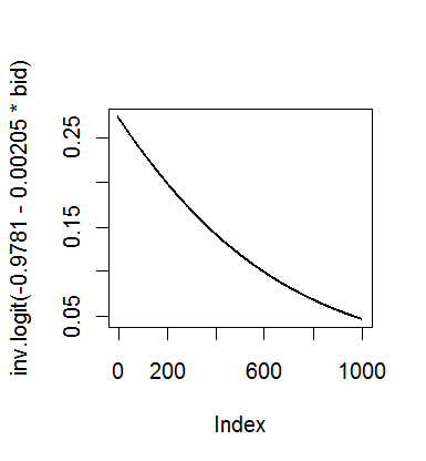
Plot output

In general, you should extract these coefficients with the coefficients command rather than transcribing them (as I did here, because I do not have access to your data).

This generalized linear model supposes the outcome associated with an independent value of $x$ has a binomial distribution whose log odds ("logit") vary linearly with $x$. The output provides the coefficients of that linear relation; namely, the intercept is estimated as -0.9781 and the slope as -0.002050. The probability, which you wish to plot, is related to the log odds by

$$\text{probability} = \frac{1}{1 + \exp(-\text{log odds})}.$$

R calls this the "inverse logit" function, inv.logit.

Putting these together gives the equation

$$\text{probability} = \frac{1}{1 + \exp\left(-[-0.9781 - 0.00205 x]\right)}.$$

An R command to plot it would be

plot(inv.logit(-0.9781 - 0.00205*(0:1000)))

Plot output

In general, you should extract these coefficients with the coefficients command rather than transcribing them (as I did here, because I do not have access to your data).

This generalized linear model supposes the outcome associated with an independent value of $x$ has a binomial distribution whose log odds ("logit") vary linearly with $x$. The output provides the coefficients of that linear relation; namely, the intercept is estimated as -0.9781 and the slope ("our_bid") as -0.002050. You can see them in the Estimate column:

              Estimate Std. Error z value Pr(>|z|)    
(Intercept) -9.781e-01  2.836e-02  -34.49   <2e-16 ***
our_bid     -2.050e-03  7.576e-05  -27.07   <2e-16 ***

The probability, which you wish to plot, is related to the log odds by

$$\text{probability} = \frac{1}{1 + \exp(-\text{log odds})}.$$

R calls this the "inverse logit" function, inv.logit.

Putting these together gives the equation

$$\text{probability} = \frac{1}{1 + \exp\left(-[-0.9781 - 0.00205 x]\right)}.$$

An R command to plot it would be

plot(inv.logit(-0.9781 - 0.00205*(0:1000)))

Plot output

In general, you should extract these coefficients with the coefficients command rather than transcribing them (as I did here, because I do not have access to your data).

added 66 characters in body
Source Link
whuber
  • 333.5k
  • 63
  • 792
  • 1.3k

This generalized linear model supposes the outcome associated with an independent value of $x$ has a binomial distribution whose log odds ("logit") vary linearly with $x$. The output provides the coefficients of that linear relation; namely, the intercept is estimated as -0.9781 and the slope as -0.002050. The probability, which you wish to plot, is related to the log odds by

$$\text{probability} = \frac{1}{1 + \exp(-\text{log odds})}.$$

R calls this the "inverse logit" function, inv.logit.

Putting these together gives the equation

$$\text{probability} = \frac{1}{1 + \exp(-0.9781 - 0.00205 x)}.$$$$\text{probability} = \frac{1}{1 + \exp\left(-[-0.9781 - 0.00205 x]\right)}.$$

An R command to plot it would be

plot(inv.logit(-0.9781 - 0.00205*(0:1000)))

Plot output

In general, you should extract these coefficients with the coefficients command rather than transcribing them (as I did here, because I do not have access to your data).

This generalized linear model supposes the outcome associated with an independent value of $x$ has a binomial distribution whose log odds ("logit") vary linearly with $x$. The output provides the coefficients of that linear relation; namely, the intercept is estimated as -0.9781 and the slope as -0.002050. The probability, which you wish to plot, is related to the log odds by

$$\text{probability} = \frac{1}{1 + \exp(-\text{log odds})}.$$

R calls this the "inverse logit" function, inv.logit.

Putting these together gives the equation

$$\text{probability} = \frac{1}{1 + \exp(-0.9781 - 0.00205 x)}.$$

An R command to plot it would be

plot(inv.logit(-0.9781 - 0.00205*(0:1000)))

In general, you should extract these coefficients with the coefficients command rather than transcribing them (as I did here, because I do not have access to your data).

This generalized linear model supposes the outcome associated with an independent value of $x$ has a binomial distribution whose log odds ("logit") vary linearly with $x$. The output provides the coefficients of that linear relation; namely, the intercept is estimated as -0.9781 and the slope as -0.002050. The probability, which you wish to plot, is related to the log odds by

$$\text{probability} = \frac{1}{1 + \exp(-\text{log odds})}.$$

R calls this the "inverse logit" function, inv.logit.

Putting these together gives the equation

$$\text{probability} = \frac{1}{1 + \exp\left(-[-0.9781 - 0.00205 x]\right)}.$$

An R command to plot it would be

plot(inv.logit(-0.9781 - 0.00205*(0:1000)))

Plot output

In general, you should extract these coefficients with the coefficients command rather than transcribing them (as I did here, because I do not have access to your data).

Source Link
whuber
  • 333.5k
  • 63
  • 792
  • 1.3k

This generalized linear model supposes the outcome associated with an independent value of $x$ has a binomial distribution whose log odds ("logit") vary linearly with $x$. The output provides the coefficients of that linear relation; namely, the intercept is estimated as -0.9781 and the slope as -0.002050. The probability, which you wish to plot, is related to the log odds by

$$\text{probability} = \frac{1}{1 + \exp(-\text{log odds})}.$$

R calls this the "inverse logit" function, inv.logit.

Putting these together gives the equation

$$\text{probability} = \frac{1}{1 + \exp(-0.9781 - 0.00205 x)}.$$

An R command to plot it would be

plot(inv.logit(-0.9781 - 0.00205*(0:1000)))

In general, you should extract these coefficients with the coefficients command rather than transcribing them (as I did here, because I do not have access to your data).