n <- 51                      # Number of interpolation points
    k.1 <- floor(n * 2/3)        # Width of the left-hand interval
    k.2 <- n - k.1               # ............ right-hand interval
    x <- seq(0, 1, length.out=n) # x coordinates
    set.seed(17)
    
    # Generate random values of the second derivative that are first negative,
    # then positive.  Modify to suit.
    y.2 <- (c(runif(k.1, -1, 0), 0.5*runif(k.2, 0, 1))) * 
                                 abs(cos(3*pi * x)) + 
      c(rep(-.1, k.1), rep(.5,k.2))
    
    # Recover the first derivative and then the transformation. 
    # Control the 
    # minimum slope of the transformation.
    y.1 <- cumsum(y.2)
    y.1 <- y.1 - min(y.1) + 0.005 * diff(range(y.1))
    y <- cumsum(y.1)
    y <- (y - y[1]) / (y[n] - y[1]) # Normalize the 
                                    # transformation
    
    #
    # Plot the graphs.
    par(mfrow=c(1,3))
    plot(x, y.2, type="l", bty="n", main="Second derivative")
    points(x, y.2, pch=20, cex=0.5)
    abline(h=0, col="Red", lty=3)
    plot(x, y.1, type="l", bty="n", lwd=2, main="First 
           derivative")
    abline(h=0, col="Red", lty=3)
    plot(x, y, type="l", lwd=2, main="Transformation")
n <- 51                      # Number of interpolation points
k.1 <- floor(n * 2/3)        # Width of the left-hand interval
k.2 <- n - k.1               # ............ right-hand interval
x <- seq(0, 1, length.out=n) # x coordinates
set.seed(17)

# Generate random values of the second derivative that are first negative,
# then positive.  Modify to suit.
y.2 <- (c(runif(k.1, -1, 0), 0.5*runif(k.2, 0, 1))) * 
                             abs(cos(3*pi * x)) + 
  c(rep(-.1, k.1), rep(.5,k.2))

# Recover the first derivative and then the transformation. 
# Control the 
# minimum slope of the transformation.
y.1 <- cumsum(y.2)
y.1 <- y.1 - min(y.1) + 0.005 * diff(range(y.1))
y <- cumsum(y.1)
y <- (y - y[1]) / (y[n] - y[1]) # Normalize the 
                                # transformation

#
# Plot the graphs.
par(mfrow=c(1,3))
plot(x, y.2, type="l", bty="n", main="Second derivative")
points(x, y.2, pch=20, cex=0.5)
abline(h=0, col="Red", lty=3)
plot(x, y.1, type="l", bty="n", lwd=2, main="First 
       derivative")
abline(h=0, col="Red", lty=3)
plot(x, y, type="l", lwd=2, main="Transformation")
added 75 characters in body
Source Link
kjetil b halvorsen
  • 82.8k
  • 32
  • 201
  • 663

[![Figure][1]][1]Figure

n
    n <- 51                      # Number of interpolation points
    k.1 <- floor(n * 2/3)        # Width of the left-hand interval
    k.2 <- n - k.1               # ............ right-hand interval
    x <- seq(0, 1, length.out=n) # x coordinates
    set.seed(17)
    
    # Generate random values of the second derivative that are first negative,
    # then positive.  Modify to suit.
    y.2 <- (c(runif(k.1, -1, 0), 0.5*runif(k.2, 0, 1))) * 
                                 abs(cos(3*pi * x)) + 
      c(rep(-.1, k.1), rep(.5,k.2))
    
    # Recover the first derivative and then the transformation. 
    # Control the 
    # minimum slope of the transformation.
    y.1 <- cumsum(y.2)
    y.1 <- y.1 - min(y.1) + 0.005 * diff(range(y.1))
    y <- cumsum(y.1)
    y <- (y - y[1]) / (y[n] - y[1]) # Normalize the 
                                    # transformation
    
    #
    # Plot the graphs.
    par(mfrow=c(1,3))
    plot(x, y.2, type="l", bty="n", main="Second derivative")
    points(x, y.2, pch=20, cex=0.5)
    abline(h=0, col="Red", lty=3)
    plot(x, y.1, type="l", bty="n", lwd=2, main="First 
           derivative")
    abline(h=0, col="Red", lty=3)
    plot(x, y, type="l", lwd=2, main="Transformation")

[![Figure][1]][1]

n

Figure

    n <- 51                      # Number of interpolation points
    k.1 <- floor(n * 2/3)        # Width of the left-hand interval
    k.2 <- n - k.1               # ............ right-hand interval
    x <- seq(0, 1, length.out=n) # x coordinates
    set.seed(17)
    
    # Generate random values of the second derivative that are first negative,
    # then positive.  Modify to suit.
    y.2 <- (c(runif(k.1, -1, 0), 0.5*runif(k.2, 0, 1))) * 
                                 abs(cos(3*pi * x)) + 
      c(rep(-.1, k.1), rep(.5,k.2))
    
    # Recover the first derivative and then the transformation. 
    # Control the 
    # minimum slope of the transformation.
    y.1 <- cumsum(y.2)
    y.1 <- y.1 - min(y.1) + 0.005 * diff(range(y.1))
    y <- cumsum(y.1)
    y <- (y - y[1]) / (y[n] - y[1]) # Normalize the 
                                    # transformation
    
    #
    # Plot the graphs.
    par(mfrow=c(1,3))
    plot(x, y.2, type="l", bty="n", main="Second derivative")
    points(x, y.2, pch=20, cex=0.5)
    abline(h=0, col="Red", lty=3)
    plot(x, y.1, type="l", bty="n", lwd=2, main="First 
           derivative")
    abline(h=0, col="Red", lty=3)
    plot(x, y, type="l", lwd=2, main="Transformation")
Source Link
whuber
  • 333.6k
  • 63
  • 792
  • 1.3k

Let me offer the most general solution consistent with the requirements: that will give you the most flexibility to choose and optimize.

We may interpret "S-shaped" as a monotonically increasing curve (because the transformation ought to be one-to-one) consisting of one part that is concave upwards and another part that is concave downwards. We may focus on making the left half concave down, because the other type (with left half concave up) is obtained through inverting such transformations.

Since the transformation $f$ is supposed to be differentiable, it must therefore have a decreasing derivative $f^\prime$ in the left half and an increasing derivative in the right half. Regardless, the derivative must be nonnegative and can be zero only at an isolated point (if at all: the minimum value of the derivative gives the least slope of the transformation.)

It is not required that the derivative be differentiable, but as a practical matter we may suppose that it is differentiable almost everywhere with derivative $f^{\prime\prime}$.

This second derivative can do practically anything: all we require is that

  • it is integrable,

  • is less than or equal to zero for all values in some left-hand interval $[0, k)$, and

  • is greater than or equal to zero for all values in the right hand interval $(k, 1]$.

Such functions $f^{\prime\prime}$ (and their inverses) parameterize the set of all solutions. (There is some redundancy: it is taken care of by a final normalization step described below.)

The Fundamental Theorem of Calculus enables us to recover $f$ from any such specification. That is,

$$f^\prime(x) = \int_0^x f^{\prime\prime}(t) dt$$

and

$$f(x) = \int_0^x f^\prime(t) dt.$$

The conditions on $f^{\prime\prime}$ guarantee that $f$ rises monotonically from its minimim $f(0)$ to some maximum $f(1) = C$. Finally, normalize $f$ by dividing the values of the preceding integral by $C$.


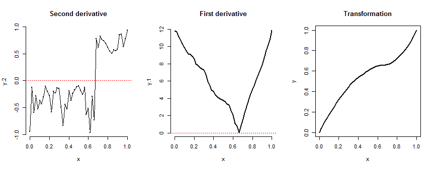
Here is an illustration starting with a version of a random walk for the second derivative. In it, the derivatives have not been normalized, but the transformation $f$ has been.

[![Figure][1]][1]

To apply this approach, you may begin with an analytic expression for $f^{\prime\prime}$, perhaps varied by a finite number of parameters. You may also specify it by giving some points along its graph and interpolating among them--provided that the interpolator respects the negativity of the values on $[0,k)$ and the positivity on $(k,1]$. The latter is the method used to generate the illustration. The corresponding R code (below) provides the details of the calculation.

This approach enables you to design any transformation you like. You could begin by sketching the S-curve, estimating its (relative) slopes $f^\prime$, and from that estimating its slopes. Specify some $f^{\prime\prime}$ to match that latter picture, then proceed to compute $f^\prime$ and then $f$.

Note that $f$ that are first concave up and then concave down can also be obtained by negating $f^{\prime\prime}$ at the outset. The critical condition for creating an S-shaped curve is that (apart from possible excursions on a set of measure zero) $f^{\prime\prime}$ may actually cross zero at most once.

Incidentally, the solution $f(x)=x$ arises by setting $f^{\prime\prime}(x)=0$ almost everywhere, making $f^\prime$ constant and positive, whence $f$ is linear; normalization assures the slope is $1$ and the intercept is $0$. (Making $f^\prime$ constant and negative produces the solution $f(x)=1-x$.)

n