###General solution

Let $f$ be the density of a symmetrical distribution with zero expectation (such as any Student $t$ distribution with $\nu \gt 1$ degrees of freedom) and $F$ be its distribution function. Integrating by parts for $\mu \ge 0$, observe that

$$\int_\mu^\infty t f(t) dt = (t(1-F(t)))\big|_\mu^\infty + \int_\mu^\infty(1-F(t))dt = \mu(1-F(\mu)) + \int_\mu^\infty(1-F(t))dt.$$

Let's call this function $h(\mu)$.

Shift the location of the distribution to $\mu \ge 0$. Let's compute its mean absolute deviation from its new mean:

$$\operatorname{MAD}(f, \mu) = \int_{-\infty}^\infty |t|f(t-\mu)dt = \int_{-\infty}^\infty |t-\mu| f(t) dt.$$

Break the latter at $0$ and $\mu$ into three integrals:

$$\eqalign{ &=\left(\int_{-\infty}^0 + \int_0^\mu + \int_{\mu}^\infty\right) |t-\mu| f(t)dt \\ &=\int_{-\infty}^0 (\mu-t)f(t)dt + \int_0^\mu (\mu-t) f(t)dt + \int_{\mu}^\infty (t-\mu) f(t)dt. }$$

Substitute $t\to -t$ in the first, expand them all, and cancel as many terms as possible:

$$\eqalign{ &=(\mu F(0) + h(0)) + (\mu(F(\mu)-F(0)) -h(0) + h(\mu)) + (h(\mu) - \mu(1-F(\mu))) \\ &= \mu(2F(\mu)-1) + 2h(\mu) \\ &= \mu + 2\int_\mu^\infty(1-F(t))dt. }$$

We will find the middle expression most convenient with the Student $t$ distribution, but the final one is rather pretty: it's the mean plus the integral of the tails of the distribution. It shows that for distributions with rapidly decreasing tails, the MAD quickly approximates the mean itself when the mean is large.

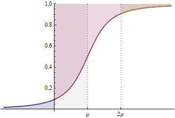
The curve plots $F$ shifted to the right by $\mu$. The MAD is the total dark shaded area: above the curve for positive values, below it for negative values. The red region between $\mu$ and $2\mu$ is congruent to the gray region beneath the curve from $0$ to $\mu$; together, they fit into the entire gray shaded rectangle of base $\mu$ and height $1$, thereby accounting for the $\mu$ term in the formula. The remaining portions are the two tail areas $\int_\mu^\infty (1-F(t))dt=\int_{-\infty}^{-\mu}F(t)dt$ which, because $F$ is symmetric around $0$, are congruent.

Let's shift the distribution to $\mu/\sigma$ and then scale it by a factor of $\sigma$. The scaling must change $\mathbb{E}(|t|)$ by a factor of $|\sigma| = \sigma$ and it scales the mean $\mu/\sigma$ to $\sigma$. The formula for the MAD of this location-scale family defined by $f$, with location $\mu$ and scale $\sigma$, therefore is

$$\operatorname{MAD}(f,\mu,\sigma) = \mu(2F(\mu/\sigma) - 1) + 2\sigma h(\mu/\sigma).\tag{1}$$

Finally, because we assumed the distribution $F$ was symmetric with zero expectation, the MAD for $\mu$ must equal the MAD for $-\mu$.

###MAD for the Student t distribution

The density function for the Student t distribution with $\nu$ degrees of freedom is

$$f_\nu(t) = \frac{\nu^{\nu/2}}{B\left(\frac{\nu}{2}, \frac{1}{2}\right)} \left(t^2 + \nu\right)^{-(1+\nu)/2} = C(\nu)\left(t^2 + \nu\right)^{-(1+\nu)/2} .$$

The inviting substitution $u = t^2+\nu$ makes short work of computing $h(\mu)$. Because $\mu \ge 0$, this is a one-to-one transformation, giving

$$\eqalign{ h(\mu) &= C(\nu)\int_\mu^\infty t (t^2 + \nu)^{-(1+\nu)/2}dt =\frac{C(\nu)}{2}\int_{\mu^2 + \nu}^\infty u^{-(1+\nu)/2}du\\ &= \frac{C(\nu)}{(\nu-1)(\mu^2 + \nu)^{(\nu-1)/2}}.}$$

For $\mu=0$ and $\sigma=1$, the symmetry implies $F(\mu/\sigma)=F(0)=1/2$, simplifying $(1)$ to

$$\operatorname{MAD}(f_\nu,0,1) = 2h(0) = \frac{2C(\nu)}{(\nu-1)\nu^{(\nu-1)/2}} = \frac{2\sqrt{\nu}}{(\nu-1)B(\nu/2, 1/2)}.$$

###Conclusions

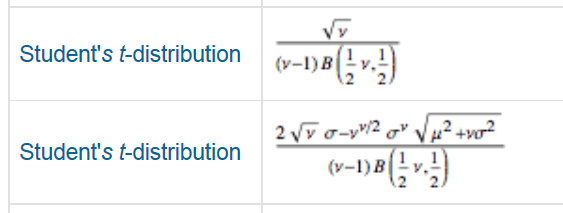
Neither $(1)$ nor the simplified version for $\mu=0, \sigma=1$ agrees with those on the Wolfram site:

The first lacks a factor of $2$. The second has multiple typographical errors. As written, it's clearly wrong because it does not scale correctly with $\sigma$: it needs to be proportional to it. The denominator is correct, but evidently some significant formatting errors occurred in the numerator.

###Verification

We may quickly compare simulated estimates of the MAD with the formula $(1)$. Here is an R implementation. In one million iterations with $\mu=-3, \sigma=4,\nu=2$ it output

Simulated   Formula 
 6.390525  6.403124 

The two values are not significantly different.

C <- function(nu) nu^(nu/2) / beta(nu/2, 1/2)
h <- function(nu, mu=0) C(nu) * (1/(nu-1) * (mu^2 + nu)^((1-nu)/2))
MAD <- function(nu, mu=0, sigma=1) {
  mu <- mu/sigma
  (mu * (2*pt(mu, nu) - 1) +  2*h(nu, mu))*sigma
}
set.seed(17)
mu <- -3
sigma <- 4
nu <- 2
c(Simulated=mean(abs(mu + sigma*rt(1e6, nu))), Formula=MAD(nu, abs(mu), sigma))