Updated images and made one clickable to reveal larger version. Tried to improve the notation a bit.
Source Link
cardinal
  • 27.3k
  • 8
  • 105
  • 140

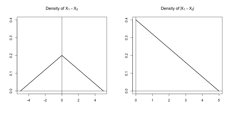
Since $X_1$ and $X_2$ are independent uniforms, then $X_1 - X_2$ has a triangular distribution, whence $Z_1 = |X_1 - X_2|$ has a distribution with density function $$ f_a(x) = \frac{2}{a^2}(a-x) ,\quad 0 < x < a \> . $$$$ f_a(z_1) = \frac{2}{a^2}(a-z_1) ,\quad 0 < z_1 < a \> . $$ The corresponding distribution function is $F_a(x) = 1 - (1-x/a)^2$$F_a(z_1) = 1 - (1-z_1/a)^2$ for $0 \leq x \leq a$$0 \leq z_1 \leq a$. Similarly, $Z_2 = |Y_1 - Y_2|$ has density $f_b(y)$$f_b(z_2)$ and distribution function $F_b(y)$$F_b(z_2)$.

Density figureTriangular densities

So $Z_1$ and $Z_2$ are independent and are supported on $[0,a]$ and $[0,b]$ respectively. For fixed $d$, the distribution function of the euclidean distance is $$\renewcommand{\Pr}{\mathbb P}\newcommand{\rd}{\,\mathrm{d}} \Pr(D \leq d) = \iint_{\{x^2+y^2 \leq d^2\}} f_a(x) f_b(y) \rd x \rd y \> . $$$$\renewcommand{\Pr}{\mathbb P}\newcommand{\rd}{\,\mathrm{d}} \Pr(D \leq d) = \iint_{\{z_1^2+z_2^2 \leq d^2\}} f_a(z_1) f_b(z_2) \rd z_1 \rd z_2 \> . $$

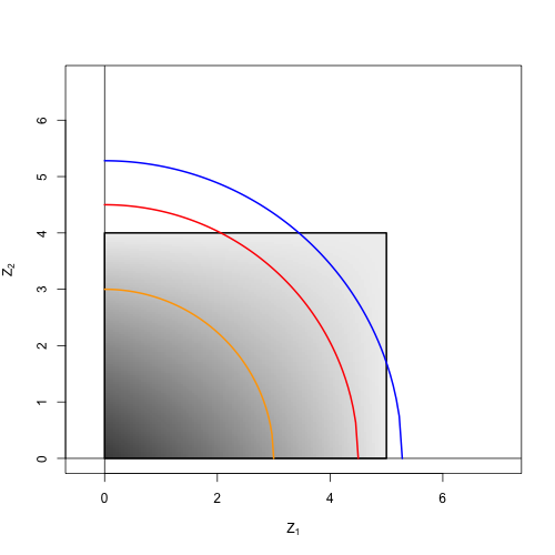
Here is a figure, where we draw an example radius of each of the three types. The rectangle is defined by $a = 5$, $b = 4$. The grayscale heatmap within the rectangle shows the density $f_a(z_1) f_b(z_2) \rd z_1 \rd z_2$ where dark areas have higher density and lighter areas have smaller density. Clicking on the figure will open a larger version of it.

Induced distribution: IntersectionsInduced distribution: Intersections

Since $X_1$ and $X_2$ are independent uniforms, then $X_1 - X_2$ has a triangular distribution, whence $Z_1 = |X_1 - X_2|$ has a distribution with density function $$ f_a(x) = \frac{2}{a^2}(a-x) ,\quad 0 < x < a \> . $$ The corresponding distribution function is $F_a(x) = 1 - (1-x/a)^2$ for $0 \leq x \leq a$. Similarly, $Z_2 = |Y_1 - Y_2|$ has density $f_b(y)$ and distribution function $F_b(y)$.

Density figure

So $Z_1$ and $Z_2$ are independent and are supported on $[0,a]$ and $[0,b]$ respectively. For fixed $d$, the distribution function of the euclidean distance is $$\renewcommand{\Pr}{\mathbb P}\newcommand{\rd}{\,\mathrm{d}} \Pr(D \leq d) = \iint_{\{x^2+y^2 \leq d^2\}} f_a(x) f_b(y) \rd x \rd y \> . $$

Here is a figure, where we draw an example radius of each of the three types. The rectangle is defined by $a = 5$, $b = 4$.

Induced distribution: Intersections

Since $X_1$ and $X_2$ are independent uniforms, then $X_1 - X_2$ has a triangular distribution, whence $Z_1 = |X_1 - X_2|$ has a distribution with density function $$ f_a(z_1) = \frac{2}{a^2}(a-z_1) ,\quad 0 < z_1 < a \> . $$ The corresponding distribution function is $F_a(z_1) = 1 - (1-z_1/a)^2$ for $0 \leq z_1 \leq a$. Similarly, $Z_2 = |Y_1 - Y_2|$ has density $f_b(z_2)$ and distribution function $F_b(z_2)$.

Triangular densities

So $Z_1$ and $Z_2$ are independent and are supported on $[0,a]$ and $[0,b]$ respectively. For fixed $d$, the distribution function of the euclidean distance is $$\renewcommand{\Pr}{\mathbb P}\newcommand{\rd}{\,\mathrm{d}} \Pr(D \leq d) = \iint_{\{z_1^2+z_2^2 \leq d^2\}} f_a(z_1) f_b(z_2) \rd z_1 \rd z_2 \> . $$

Here is a figure, where we draw an example radius of each of the three types. The rectangle is defined by $a = 5$, $b = 4$. The grayscale heatmap within the rectangle shows the density $f_a(z_1) f_b(z_2) \rd z_1 \rd z_2$ where dark areas have higher density and lighter areas have smaller density. Clicking on the figure will open a larger version of it.

Induced distribution: Intersections

Fixed some typos in the math. I'm sure there are others.
Source Link
cardinal
  • 27.3k
  • 8
  • 105
  • 140

Now, the inner integral yields $\frac{1}{a^2}\radius (2 a - \radius)$. So, we are left to compute an integral of the form $$ G(c) - G(0) = \int_0^c (b - y) \radius (2b - \radius) \rd y \> , $$$$ G(c) - G(0) = \int_0^c (b - y) \radius (2a - \radius) \rd y \> , $$ where in this case of interest $c = d$. The antiderivative of the integrand is $$ \begin{align*} G(y) &= \int (b - y) \radius (2b - \radius) \rd y \\ &= \frac{a}{3} \radius ( y (3 b - 2 y) + 2 d^2) \\ &\quad + \,a b d^2 \tan^{-1}(x / \radius) - b d^2 x \\ &\quad + \,\frac{b y^3}{3} + \frac{(d y)^2}{2} - \frac{y^4}{4} \> . \end{align*} $$$$ \begin{align*} G(y) &= \int (b - y) \radius (2a - \radius) \rd y \\ &= \frac{a}{3} \radius ( y (3 b - 2 y) + 2 d^2) \\ &\quad + \,a b d^2 \tan^{-1}\Big(\frac{y}{{\scriptstyle \radius}}\Big) - b d^2 y \\ &\quad + \,\frac{b y^3}{3} + \frac{(d y)^2}{2} - \frac{y^4}{4} \> . \end{align*} $$

Now, the inner integral yields $\frac{1}{a^2}\radius (2 a - \radius)$. So, we are left to compute an integral of the form $$ G(c) - G(0) = \int_0^c (b - y) \radius (2b - \radius) \rd y \> , $$ where in this case of interest $c = d$. The antiderivative of the integrand is $$ \begin{align*} G(y) &= \int (b - y) \radius (2b - \radius) \rd y \\ &= \frac{a}{3} \radius ( y (3 b - 2 y) + 2 d^2) \\ &\quad + \,a b d^2 \tan^{-1}(x / \radius) - b d^2 x \\ &\quad + \,\frac{b y^3}{3} + \frac{(d y)^2}{2} - \frac{y^4}{4} \> . \end{align*} $$

Now, the inner integral yields $\frac{1}{a^2}\radius (2 a - \radius)$. So, we are left to compute an integral of the form $$ G(c) - G(0) = \int_0^c (b - y) \radius (2a - \radius) \rd y \> , $$ where in this case of interest $c = d$. The antiderivative of the integrand is $$ \begin{align*} G(y) &= \int (b - y) \radius (2a - \radius) \rd y \\ &= \frac{a}{3} \radius ( y (3 b - 2 y) + 2 d^2) \\ &\quad + \,a b d^2 \tan^{-1}\Big(\frac{y}{{\scriptstyle \radius}}\Big) - b d^2 y \\ &\quad + \,\frac{b y^3}{3} + \frac{(d y)^2}{2} - \frac{y^4}{4} \> . \end{align*} $$

Source Link
cardinal
  • 27.3k
  • 8
  • 105
  • 140

We can solve this problem analytically using some geometric intuition and arguments. Unfortunately, the answer is quite long and a bit messy.

Basic setup

First, let's set out some notation. Assume we draw points uniformly at random from the rectangle $[0,a] \times [0,b]$. We assume without loss of generality that $0 < b < a$. Let $(X_1,Y_1)$ be the coordinates of the first point and $(X_2,Y_2)$ be the coordinates of the second point. Then, $X_1$, $X_2$, $Y_1$, and $Y_2$ are mutually independent with $X_i$ distributed uniformly on $[0,a]$ and $Y_i$ distributed uniformly on $[0,b]$.

Consider the Euclidean distance between the two points. This is $$ D = \sqrt{(X_1-X_2)^2 + (Y_1-Y_2)^2} =: \sqrt{ Z_1^2 + Z_2^2} \> , $$ where $Z_1 = |X_1-X_2|$ and $Z_2 = |Y_1-Y_2|$.

Triangular distributions

Since $X_1$ and $X_2$ are independent uniforms, then $X_1 - X_2$ has a triangular distribution, whence $Z_1 = |X_1 - X_2|$ has a distribution with density function $$ f_a(x) = \frac{2}{a^2}(a-x) ,\quad 0 < x < a \> . $$ The corresponding distribution function is $F_a(x) = 1 - (1-x/a)^2$ for $0 \leq x \leq a$. Similarly, $Z_2 = |Y_1 - Y_2|$ has density $f_b(y)$ and distribution function $F_b(y)$.

Note that since $Z_1$ is a function only of the two $X_i$ and $Z_2$ is a function only of the $Y_i$, then $Z_1$ and $Z_2$ are independent. So the distance between the points is the euclidean norm of two independent random variables (with different distributions).

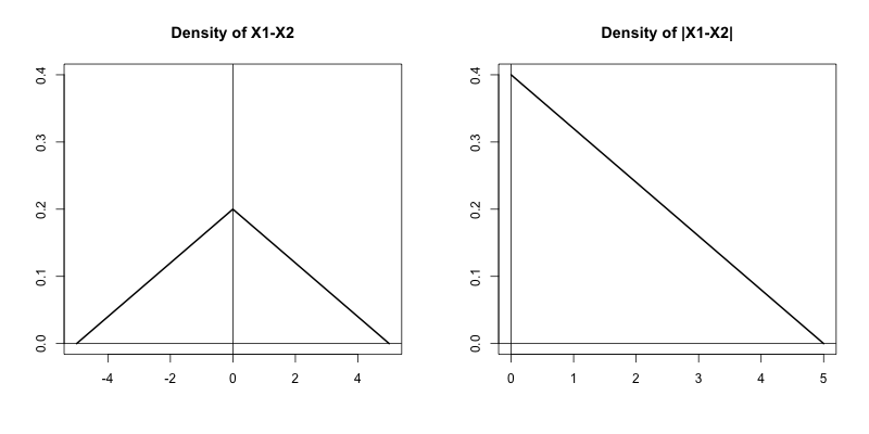
The left panel of the figure shows the distribution of $X_1 - X_2$ and the right panel shows $Z_1 = |X_1 - X_2|$ where $a = 5$ in this example.
Density figure

Some geometric probability

So $Z_1$ and $Z_2$ are independent and are supported on $[0,a]$ and $[0,b]$ respectively. For fixed $d$, the distribution function of the euclidean distance is $$\renewcommand{\Pr}{\mathbb P}\newcommand{\rd}{\,\mathrm{d}} \Pr(D \leq d) = \iint_{\{x^2+y^2 \leq d^2\}} f_a(x) f_b(y) \rd x \rd y \> . $$

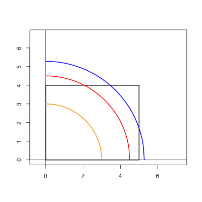
We can think of this geometrically as having a distribution on the rectangle $[0,a] \times [0,b]$ and considering a quarter circle of radius $d$. We'd like to know the probability that is inside the intersection of these two regions. There are three different possibilities to consider:

Region 1 (orange): $0 \leq d < b$. Here the quarter circle lies completely within the rectangle.

Region 2 (red): $b \leq d \leq a$. Here the quarter circle intersects the rectange along the top and bottom edges.

Region 3 (blue): $a < d \leq \sqrt{a^2 + b^2}$. The quarter circle intersects the rectangle along the top and right edges.

Here is a figure, where we draw an example radius of each of the three types. The rectangle is defined by $a = 5$, $b = 4$.
Induced distribution: Intersections

Some ugly calculus

To calculate the probabilities, we need to do some calculus. Let's consider each of the regions in turn and we'll see that a common integral will arise. This integral has a closed-form, though it's not very pretty.

Region 1: $0 \leq d < b$.

$$\newcommand{\radius}{\sqrt{d^2 - y^2}} \Pr(D \leq d) = \int_0^d \int_0^{\radius} f_b(y) f_a(x) \rd x \rd y = \int_0^d f_b(y) \int_0^{\radius} f_a(x) \rd x \rd y \>. $$

Now, the inner integral yields $\frac{1}{a^2}\radius (2 a - \radius)$. So, we are left to compute an integral of the form $$ G(c) - G(0) = \int_0^c (b - y) \radius (2b - \radius) \rd y \> , $$ where in this case of interest $c = d$. The antiderivative of the integrand is $$ \begin{align*} G(y) &= \int (b - y) \radius (2b - \radius) \rd y \\ &= \frac{a}{3} \radius ( y (3 b - 2 y) + 2 d^2) \\ &\quad + \,a b d^2 \tan^{-1}(x / \radius) - b d^2 x \\ &\quad + \,\frac{b y^3}{3} + \frac{(d y)^2}{2} - \frac{y^4}{4} \> . \end{align*} $$

From this we get that $\Pr(D \leq d) = \frac{2}{a^2 b^2} (G(d) - G(0))$.

Region 2: $b \leq d \leq a$.

$$ \Pr(D \leq d) = \frac{2}{a^2 b^2} (G(b) - G(0)) \>, $$ by the same reasoning as for Region 1, except now we must integrate along the $y$-axis all the way up to $b$ instead of just $d$.

Region 3: $a < d \leq \sqrt{a^2 + b^2}$. $$ \begin{align*} \Pr(D \leq d) &= \int_0^\sqrt{d^2-a^2} f_b(y)\rd y + \int_{\sqrt{d^2-a^2}}^b f_b(y) \int_{0}^\radius f_a(x) \rd x \rd y \\ &= F_b(\sqrt{d^2-a^2}) + \frac{2}{a^2 b^2} (G(b) - G(\sqrt{d^2-a^2})) \end{align*} $$

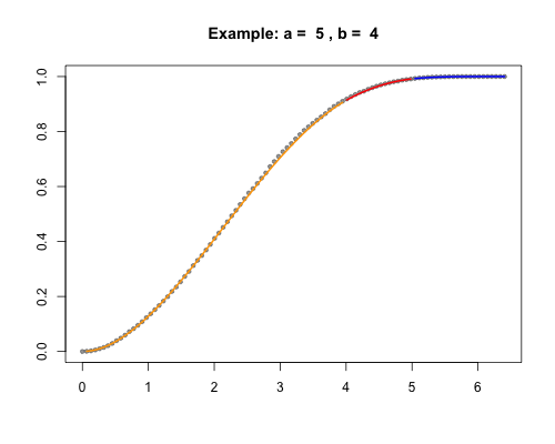
Below is a simulation of 20000 points where we plot the empirical distribution as grey points and the theoretical distribution as a line, colored according to the particular region that applies.
Empirical cdf and theoretical

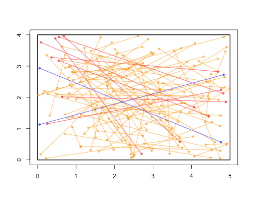
From the same simulation, below we plot the first 100 pairs of points and draw lines between them. Each is colored according to the distance between the pair of points and which region this distance falls into.
Random sample of points

The expected number of pairs of points within distance $d$ is simply $$ \mathbb E[\xi] = {n \choose 2} \Pr(D \leq d) \>, $$ by linearity of expectation.