replaced http://stats.stackexchange.com/ with https://stats.stackexchange.com/
Source Link
Introduce rma tool
Source Link
jwimberley
  • 4k
  • 2
  • 14
  • 20

SECOND EDIT

The other answer from the same previous question by @Wolfgang gives an even better solution: the rma tool from the metafor package (I originally interpreted text in that answer to mean that it did not calculate the intercept, but that's not the case). Taking the variances in the measurements y to be simply y:

> rma(y~x+I(x^2),y,method="FE")

Fixed-Effects with Moderators Model (k = 10)

Test for Residual Heterogeneity: 
QE(df = 7) = 8.2817, p-val = 0.3084

Test of Moderators (coefficient(s) 2,3): 
QM(df = 2) = 659.4641, p-val < .0001

Model Results:

         estimate       se     zval    pval    ci.lb     ci.ub     
intrcpt   46.6629  16.0838   2.9012  0.0037  15.1393   78.1866   **
x         88.1940   8.0956  10.8940  <.0001  72.3268  104.0612  ***
I(x^2)    -3.9140   0.7803  -5.0161  <.0001  -5.4433   -2.3847  ***

---
Signif. codes:  0 ‘***’ 0.001 ‘**’ 0.01 ‘*’ 0.05 ‘.’ 0.1 ‘ ’ 1

This is definitely the best pure R tool for this type of regression that I've found.

Showing a quadratic fit
Source Link
jwimberley
  • 4k
  • 2
  • 14
  • 20
import ROOT
from array import array
import math
x = range(1,11)
xerrs = [0]*10
y = [131.4,227.1,245,331.2,386.9,464.9,476.3,512.2,510.8,532.9]
yerrs = [math.sqrt(i) for i in y]
graph = ROOT.TGraphErrors(len(x),array('d',x),array('d',y),array('d',xerrs),array('d',yerrs))
graph.Fit("pol1""pol2","S")
c = ROOT.TCanvas("test","test",800,600)
graph.Draw("AP")
c.Draw()
Welcome to JupyROOT 6.07/03

****************************************
Minimizer is Linear
Chi2                      =      33 8.44322817
NDf                       =            87
p0                        =      11046.3256629   +/-   916.880040838     
p1                        =      48 88.7638194   +/-   18.936209565     
p2                        =     -3.91398   +/-   0.78028    

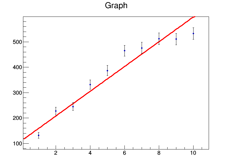
(clearly a bad fit if you count the degrees of freedom) and a nice plot is produced:

fitquadfit

import ROOT
from array import array
import math
x = range(1,11)
xerrs = [0]*10
y = [131.4,227.1,245,331.2,386.9,464.9,476.3,512.2,510.8,532.9]
yerrs = [math.sqrt(i) for i in y]
graph = ROOT.TGraphErrors(len(x),array('d',x),array('d',y),array('d',xerrs),array('d',yerrs))
graph.Fit("pol1","S")
c = ROOT.TCanvas("test","test",800,600)
graph.Draw("AP")
c.Draw()
****************************************
Minimizer is Linear
Chi2                      =      33.4432
NDf                       =            8
p0                        =      110.325   +/-   9.88004     
p1                        =      48.7638   +/-   1.9362 

(clearly a bad fit if you count the degrees of freedom) and a nice plot is produced:

fit

import ROOT
from array import array
import math
x = range(1,11)
xerrs = [0]*10
y = [131.4,227.1,245,331.2,386.9,464.9,476.3,512.2,510.8,532.9]
yerrs = [math.sqrt(i) for i in y]
graph = ROOT.TGraphErrors(len(x),array('d',x),array('d',y),array('d',xerrs),array('d',yerrs))
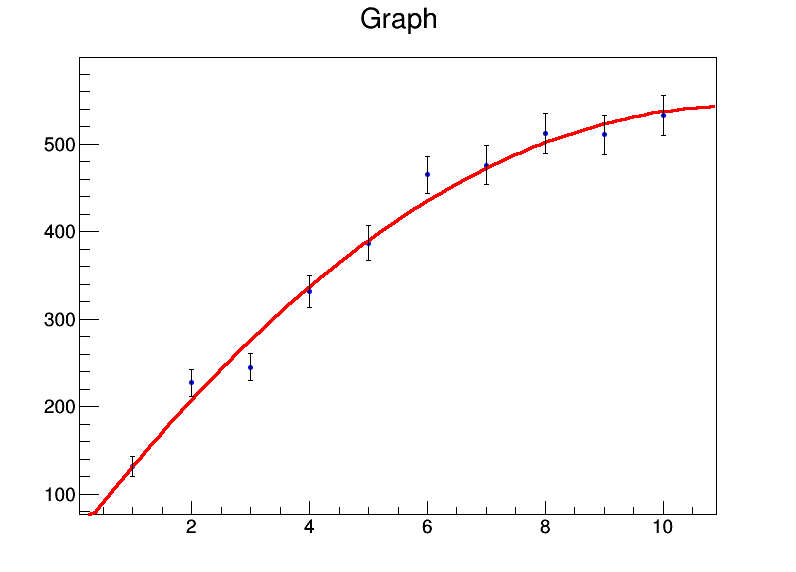
graph.Fit("pol2","S")
c = ROOT.TCanvas("test","test",800,600)
graph.Draw("AP")
c.Draw()
Welcome to JupyROOT 6.07/03

****************************************
Minimizer is Linear
Chi2                      =       8.2817
NDf                       =            7
p0                        =      46.6629   +/-   16.0838     
p1                        =       88.194   +/-   8.09565     
p2                        =     -3.91398   +/-   0.78028    

and a nice plot is produced:

quadfit

Adding a ROOT example
Source Link
jwimberley
  • 4k
  • 2
  • 14
  • 20
Loading
One final clarification regarding relative values of weights
Source Link
jwimberley
  • 4k
  • 2
  • 14
  • 20
Loading
A few more typos
Source Link
jwimberley
  • 4k
  • 2
  • 14
  • 20
Loading
Typo
Source Link
jwimberley
  • 4k
  • 2
  • 14
  • 20
Loading
Source Link
jwimberley
  • 4k
  • 2
  • 14
  • 20
Loading