added 1897 characters in body
Source Link
B_Miner
  • 8.9k
  • 22
  • 94
  • 154

ADD #3 Adds in simulation of Y0 at each sim, versus a static set

poisson.power.1cov<-function(alpha=0.05,nsims=NULL,n0=NULL,n1=NULL, covariate_mu=NULL, B0=NULL, B1=NULL, possible.effects=NULL )
{
  #hold power estimates for each effect
  powers <- rep(NA, length(possible.effects)) 
 
  #treatment indicator
  treat<-c(rep(0,n0),rep(1,n1))
  
  for (i in 1: length(possible.effects)) #loop over effects sizes
  {
      hold_power<-c()
    
      for (j in 1:nsims)
      {
        
        #simulate Y0
        Y0<-rpois((n0+n1),lambda = covariate_mu)
        #linear predictor using assumed B0, B1 and the simulated covariate Y0
        lin_pred<-B0+B1*Y0+log(possible.effects[i])*treat 
        
        #exponentiate
        mu<-exp(lin_pred)
       
        #simulate Y1 based on mu (so here we are creating n0+n1 Y1 values, each of which has a different mu)
        Y1<-rpois(n=length(mu),lambda = mu)
        
        #fit model
        mod<-glm(as.integer(Y1)~as.integer(Y0)+treat,family=poisson)
  
        #extract p-value
        sum_mod <-summary(mod)
        hold_power<-rbind(hold_power,sum_mod$coefficients[3,4])
        
      } #loop sims
    powers[i]<-mean(hold_power < alpha)
  
    } #loop effects
  
  return(powers)
  
}

#effects of interest
effects<-seq(from=1.01, to=1.20, by=0.01)
#determined from aprior data
covariate_mu <-505
#run power analysis with fixed B0 and B1
powers<-poisson.power.1cov(alpha = 0.05,n0 = 15,n1 = 15,nsims = 1000,covariate_mu =covariate_mu , B0 = 5.083739, B1 = 0.002056, possible.effects = effects)

#plot
plot(effects,powers)
lines(effects,rep(0.8,length(effects)))
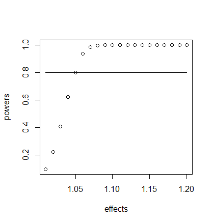
added 1991 characters in body
Source Link
B_Miner
  • 8.9k
  • 22
  • 94
  • 154

ADD #2

Here is another take at this which I believe is closer to Greg's point about $Y_{1}$ not having any randomness except as inherited from $Y_{0}$

poisson.power.1cov<-function(alpha=0.05,nsims=NULL,n0=NULL,n1=NULL, covariate=NULL, B0=NULL, B1=NULL, possible.effects=NULL )
{
  #hold power estimates for each effect
  powers <- rep(NA, length(possible.effects)) 
 
  #treatment indicator
  treat<-c(rep(0,n0),rep(1,n1))
  
  for (i in 1: length(possible.effects)) #loop over effects sizes
  {
      hold_power<-c()
    
      for (j in 1:nsims)
      {
        #linear predictor using assumed B0, B1 and the simulated covariate Y0
        lin_pred<-B0+B1*Y0+log(possible.effects[i])*treat 
        
        #exponentiate
        mu<-exp(lin_pred)
       
        #simulate Y1 based on mu (so here we are creating n0+n1 Y1 values, each of which has a different mu)
        Y1<-rpois(n=length(mu),lambda = mu)
        
        #fit model
        mod<-glm(as.integer(Y1)~as.integer(Y0)+treat,family=poisson)
  
        #extract p-value
        sum_mod <-summary(mod)
        hold_power<-rbind(hold_power,sum_mod$coefficients[3,4])
        
      } #loop sims
    powers[i]<-mean(hold_power < alpha)
  
    } #loop effects
  
  return(powers)
  
}

#effects of interest
effects<-seq(from=1.01, to=1.20, by=0.01)
#determined from aprior data
Y0<-as.integer(rpois(30,505))
#run power analysis with fixed B0 and B1
powers<-poisson.power.1cov(alpha = 0.05,n0 = 15,n1 = 15,nsims = 1000,covariate = Y0, B0 = 5.083739, B1 = 0.002056, possible.effects = effects)

#plot
plot(effects,powers)
lines(effects,rep(0.8,length(effects)))

Which yields:

enter image description here

ADD #2

Here is another take at this which I believe is closer to Greg's point about $Y_{1}$ not having any randomness except as inherited from $Y_{0}$

poisson.power.1cov<-function(alpha=0.05,nsims=NULL,n0=NULL,n1=NULL, covariate=NULL, B0=NULL, B1=NULL, possible.effects=NULL )
{
  #hold power estimates for each effect
  powers <- rep(NA, length(possible.effects)) 
 
  #treatment indicator
  treat<-c(rep(0,n0),rep(1,n1))
  
  for (i in 1: length(possible.effects)) #loop over effects sizes
  {
      hold_power<-c()
    
      for (j in 1:nsims)
      {
        #linear predictor using assumed B0, B1 and the simulated covariate Y0
        lin_pred<-B0+B1*Y0+log(possible.effects[i])*treat 
        
        #exponentiate
        mu<-exp(lin_pred)
       
        #simulate Y1 based on mu (so here we are creating n0+n1 Y1 values, each of which has a different mu)
        Y1<-rpois(n=length(mu),lambda = mu)
        
        #fit model
        mod<-glm(as.integer(Y1)~as.integer(Y0)+treat,family=poisson)
  
        #extract p-value
        sum_mod <-summary(mod)
        hold_power<-rbind(hold_power,sum_mod$coefficients[3,4])
        
      } #loop sims
    powers[i]<-mean(hold_power < alpha)
  
    } #loop effects
  
  return(powers)
  
}

#effects of interest
effects<-seq(from=1.01, to=1.20, by=0.01)
#determined from aprior data
Y0<-as.integer(rpois(30,505))
#run power analysis with fixed B0 and B1
powers<-poisson.power.1cov(alpha = 0.05,n0 = 15,n1 = 15,nsims = 1000,covariate = Y0, B0 = 5.083739, B1 = 0.002056, possible.effects = effects)

#plot
plot(effects,powers)
lines(effects,rep(0.8,length(effects)))

Which yields:

enter image description here

added 854 characters in body
Source Link
B_Miner
  • 8.9k
  • 22
  • 94
  • 154

I am interested in a power analysis for a Poisson regression of the form:

$Y_{i,1} = \beta_{0}+\beta_{1}Y_{i,0}+\beta_{2}Z_{i}$

where...

$Y_{i,1} $=The count from the 'post period' for case $i$

$Y_{i,0} $=The count from the 'pre period' for case $i$

$Z_{i} $=An indicator (0 or 1) of treatment for case $i$

There are $n_{0}$ and $n_{1}$ samples from each the control and treatment cases respectively.

I am wondering how to best simulate for a power analysis? What I know:

  • We need to declare a minimally important effect size in terms of a multiplier for the treatment, the $\beta_{2}$. Lets say this is a six percent increase on average so effect is log(1.06)
  • I do have data without a treatment and ran the model above with the treatment indicator and have the parameter estimates $\beta_{0}$ = 5.083739 and $\beta_{1}$ = 0.002056
  • Since I have the values of $Y_{i,0}$ from the time without a treatment, I could use fitdist() in R for example to estimate the parameters of this data in say a poisson

Question: What uncertainty needs to be captured in a power analysis like this?

Is it sufficient to do the following (repeated nsim times) or is this not capturing enough uncertainty by using the static values of $\beta_{0}$ and $\beta_{1}$ ? If not how?

#loop this nsims times
n0<-30
n1<-30
B0<-5.083739
B1<-0.002056
effect<-1.06

#treatment indicator
treat<-c(rep(0,n0),rep(1,n1))

#sample of values for the "pre-period" based on prior data this is how the pre-period is distributed
Y0<-as.integer(rpois(n0+n1,505))

lin_pred<-B0+B1*Y0+log(effect)*treat
Y1<-as.integer(exp(lin_pred))

mod<-glm(Y1~Y0+treat,family=poisson)
#extract the p-value from here
summary(mod) 

ADD #1

To Greg's questions, the data is paired in the sense that the same units (geographical units such as markets) are measured twice. $Y_{i,1}$ is the response variable after the intervention period (only some markets are treated of course) and $Y_{i,0}$ is the value before the intervention period....a "Pre-test" sometimes called.

This methodology comes from Google's Data Science team here and Andrew Gelman (Here)

a snippet of the former is:

enter image description here

a snippet of this later reference is:

enter image description here

I am interested in a power analysis for a Poisson regression of the form:

$Y_{i,1} = \beta_{0}+\beta_{1}Y_{i,0}+\beta_{2}Z_{i}$

where...

$Y_{i,1} $=The count from the 'post period' for case $i$

$Y_{i,0} $=The count from the 'pre period' for case $i$

$Z_{i} $=An indicator (0 or 1) of treatment for case $i$

There are $n_{0}$ and $n_{1}$ samples from each the control and treatment cases respectively.

I am wondering how to best simulate for a power analysis? What I know:

  • We need to declare a minimally important effect size in terms of a multiplier for the treatment, the $\beta_{2}$. Lets say this is a six percent increase on average so effect is log(1.06)
  • I do have data without a treatment and ran the model above with the treatment indicator and have the parameter estimates $\beta_{0}$ = 5.083739 and $\beta_{1}$ = 0.002056
  • Since I have the values of $Y_{i,0}$ from the time without a treatment, I could use fitdist() in R for example to estimate the parameters of this data in say a poisson

Question: What uncertainty needs to be captured in a power analysis like this?

Is it sufficient to do the following (repeated nsim times) or is this not capturing enough uncertainty by using the static values of $\beta_{0}$ and $\beta_{1}$ ? If not how?

#loop this nsims times
n0<-30
n1<-30
B0<-5.083739
B1<-0.002056
effect<-1.06

#treatment indicator
treat<-c(rep(0,n0),rep(1,n1))

#sample of values for the "pre-period" based on prior data this is how the pre-period is distributed
Y0<-as.integer(rpois(n0+n1,505))

lin_pred<-B0+B1*Y0+log(effect)*treat
Y1<-as.integer(exp(lin_pred))

mod<-glm(Y1~Y0+treat,family=poisson)
#extract the p-value from here
summary(mod) 

ADD #1

To Greg's questions, the data is paired in the sense that the same units (geographical units such as markets) are measured twice. $Y_{i,1}$ is the response variable after the intervention period (only some markets are treated of course) and $Y_{i,0}$ is the value before the intervention period....a "Pre-test" sometimes called.

This methodology comes from Google's Data Science team here and Andrew Gelman (Here)

a snippet of the former is:

enter image description here

a snippet of this later reference is:

enter image description here

Source Link
B_Miner
  • 8.9k
  • 22
  • 94
  • 154
Loading